
Surveys · Foundations and history
Seasonal and Temporal Effects in Repeated Cross-Sectional Surveys
When a survey is repeated over time, the date of fieldwork can change the answers as much as any real shift in opinion or behaviour. This article explains the main seasonal and temporal effects, how to recognise them, and how to design and analyse repeated surveys so that trends reflect genuine change.
Repeated cross-sectional surveys, which ask the same questions of a fresh sample at regular intervals, are the backbone of trend measurement. Monthly labour force surveys, quarterly customer satisfaction trackers, annual employee surveys and weekly political polls all rely on the same idea: if the method stays constant, differences between rounds reflect real change in the population (Firebaugh, 1997).
The method, however, never quite stays constant, because time itself is part of it. Each round is carried out in a different season, on different days, in a different news environment and sometimes by a slightly different fieldwork process. These temporal effects can create apparent changes that have nothing to do with the trend a researcher wants to measure, or hide changes that are real. This article describes the main kinds of temporal effect, the evidence on how large they are, and the design and analysis techniques that keep them under control.
Why timing matters
A survey estimate for a given round can be thought of as the sum of several components: the long-term trend in the population, regular seasonal patterns, the effect of specific events around the time of fieldwork, effects of the fieldwork process itself, and random sampling error. A naive comparison between two rounds mixes all of these. A rise in reported satisfaction from the first quarter to the second may be genuine improvement, a seasonal pattern that recurs every year, a reaction to a widely publicised event, a change in which kinds of people were reached, or chance.
Separating these components is not merely a statistical nicety. Decisions are made on the basis of reported trends. A retailer that reads a seasonal dip in customer satisfaction as a decline in service quality may change staff or policies unnecessarily, while one that attributes a real decline to the season may miss a problem until it is too late.
Seasonal effects
Many quantities measured in surveys genuinely vary with the season. Employment rises and falls with agriculture, construction, tourism and holiday retail. Spending on heating, travel and gifts follows the calendar. Health surveys find seasonal patterns in illness and physical activity. When a survey measures such quantities, seasonal variation is real, but it is usually not what users want to know. The question "is unemployment rising?" is really a question about whether it is higher than would normally be expected at this time of year.
Official statistical agencies address this through seasonal adjustment. Using several years of data, they estimate the typical seasonal pattern for each month or quarter and remove it, so that the adjusted series shows the underlying trend and irregular movements. The best-known family of methods descends from the X-11 procedure developed at the United States Census Bureau and refined in later versions such as X-12-ARIMA (Findley et al., 1998). Ladiray and Quenneville (2001) give a detailed account of how these methods separate trend, seasonal and irregular components. Alternative approaches based on local regression, such as STL decomposition, are widely used in business analytics (Cleveland et al., 1990; Hyndman & Athanasopoulos, 2021).
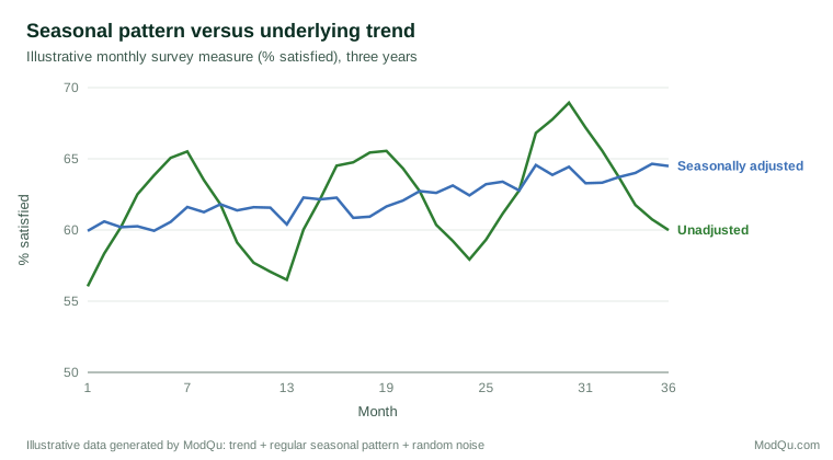
Seasonal adjustment requires a long enough series, typically at least three years of consistent monthly or quarterly data, and it assumes that the seasonal pattern is reasonably stable. When a series is short, or when an unusual year disrupts the pattern, comparisons with the same period in the previous year are a simple and transparent alternative.
Seasonality also affects attitudes and subjective measures, though usually less than people assume. Reported mood and life satisfaction vary with the day of the week: one large analysis of daily survey data from the United States found better moods on weekends and smaller differences among weekdays than the popular idea of "Blue Monday" suggests (Stone et al., 2012). An early experiment found that people interviewed by telephone on sunny days reported higher life satisfaction than those interviewed on rainy days, unless their attention was drawn to the weather (Schwarz & Clore, 1983). A much larger later study, however, using data from more than a million respondents, found that day-to-day weather had very little effect on reported life satisfaction (Lucas & Lawless, 2013). Measures of momentary experience, such as how people felt yesterday, are more sensitive to timing than global evaluations of life as a whole (Kahneman & Krueger, 2006), so it is worth recording the day and time of each interview when wellbeing is measured. The broader lesson is that transient conditions can influence subjective answers, but their average effect over a large, well-spread sample is usually small.
Calendar and fieldwork timing effects
Beyond the seasons, the precise timing of fieldwork matters for practical reasons.
Who can be reached when. People are not equally available at all times. Interviewer-administered surveys reach more households in the evening and at weekends, and those reached in the daytime on weekdays are more likely to be retired, at home with children or out of work (Weeks et al., 1987; Groves & Couper, 1998). If the fieldwork schedule changes between rounds, for example because of a holiday or a staffing shortage, the mix of respondents can change too. Online surveys face the same issue in a different form: invitations sent on a Monday morning and left open for two days reach a different group from those sent on a Friday afternoon.
Holidays and special periods. Fieldwork that overlaps with public holidays, school breaks or major sporting events may reach fewer people, and different people, than usual. Consumer surveys conducted just before major gift-giving holidays may capture spending intentions that do not reflect the rest of the year.
Early and late respondents. Within each round, people who respond quickly differ from those who respond only after reminders. Follow-up efforts bring in harder-to-reach people, which can reduce nonresponse bias, though the late respondents sometimes provide less accurate answers (Olson, 2013). If one round has a longer fieldwork period or more reminders than another, the composition of respondents and therefore the estimates can shift.
Event effects
Surveys are also affected by what is happening in the world when they are in the field. A major news story, a product recall, an economic shock or a natural disaster can change attitudes quickly, sometimes temporarily. Political polling provides the clearest examples. Analyses of election campaigns show that voter preferences move in response to conventions, debates and other events, and that much of this movement fades over the following weeks (Erikson & Wlezien, 2012). The 2016 United States presidential polls illustrate the risk of timing: an evaluation found that late shifts in preference among voters who decided in the final days contributed to errors in polls completed earlier (Kennedy et al., 2018).
For business surveys, events may be specific to the organisation or its market: a price change, a service outage, a competitor's launch or a news story about the brand. A tracking study that happens to be in the field during such an event will capture its effect, which is valuable if recognised and misleading if not. Recording the main events around each round of fieldwork, and noting them alongside the results, is a simple and effective safeguard.
When a change is deliberately introduced at a known time, such as a new service policy, the timing of surveys can be used to evaluate it. Interrupted time series analysis compares the trend before and after the change, taking account of seasonality and pre-existing trends, and provides a much stronger test than a simple before-and-after comparison (Lopez Bernal et al., 2017).
Methodological changes over time
Some of the most damaging temporal effects come not from the world but from the survey itself. Over the years, survey organisations change sampling frames, modes, questionnaire layouts, contractors and weighting procedures. Each change can introduce a break in the series. Response rates also drift: Curtin et al. (2005) documented a long decline in response to the University of Michigan's Survey of Consumers and showed that the effort required to complete each interview rose sharply over time. The study also found that the decline had surprisingly little effect on the main consumer sentiment estimates, but that cannot be assumed for every survey.
Another source of drift arises when the same organisation surveys the same population repeatedly. Different pollsters measuring the same thing often differ by a stable amount, known as a house effect, because of their particular methods. Jackman (2005) showed how house effects can be estimated and allowed for when combining polls conducted at different times by different organisations. Within a single organisation's series, a change in method can create an equivalent shift partway through the series.
The safest response is to change methods rarely and deliberately, and to measure the effect of any change. When a mode or questionnaire must change, running the old and new versions side by side with random subsamples for at least one round allows the size of the break to be estimated and the series to be bridged.
Period, age and cohort over the long run
Over longer spans of time, a repeated cross-section captures three intertwined influences. Period effects are changes that affect everyone at a particular time, such as a recession or a new technology. Age effects are changes that come with getting older. Cohort effects are lasting differences between generations shaped by the conditions in which they grew up. Ryder (1965) argued that much social change happens as one cohort replaces another, so that a population's average attitudes can change even if no individual changes their mind.
A long series of repeated cross-sections is the main source of evidence for distinguishing these influences, because it observes people of every age at many different times. The task is harder than it looks: birth year, age and calendar year are linked, so the three effects cannot be separated by statistical modelling alone without some assumptions about which of them is absent or follows a particular shape (Glenn, 2005). For practical users, the point is that a long-term rise in a survey measure may reflect generational turnover rather than any change in how individuals think, which matters when deciding whether a trend is likely to continue or reverse.
A worked example
Consider a company that surveys a fresh random sample of 600 employees each quarter and reports the share who say they are likely to stay for another year. Over two years the figures are 71%, 66%, 72% and 70% in the first year and 70%, 64%, 71% and 69% in the second. A manager reading only the latest two quarters sees a fall from 71% to 69% and asks what went wrong.
Three checks put the change in context. First, the sampling error on a difference between two independent samples of 600 at around 70% is about ±5 points, so a two-point fall is well within chance. Second, comparing each quarter with the same quarter a year earlier shows changes of only one or two points, suggesting broad stability. Third, the second quarter is lower in both years, a pattern that turns out to coincide with the annual pay review, when dissatisfaction is temporarily higher. The apparent decline is a mixture of chance and a recurring seasonal dip. What would deserve attention is a second-quarter figure well below 64%, or a fall that persisted into the next quarter.
Designing repeated surveys to control temporal effects
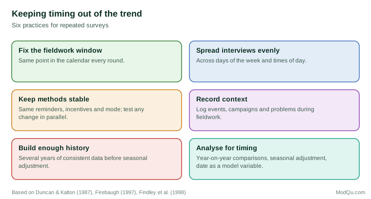
Several design choices reduce the risk that timing will distort trends (Duncan & Kalton, 1987; Firebaugh, 1997):
- Fix the fieldwork window. Conduct each round at the same point in the calendar, for example the second and third weeks of each quarter, so that seasonal and calendar influences are similar across rounds.
- Spread interviews evenly. Distribute invitations and interviewer effort evenly across days of the week and times of day, so that no single day or event dominates a round.
- Keep the process stable. Hold the number of reminders, the length of the fieldwork period and the incentive constant between rounds, so that the mix of early and late respondents remains comparable.
- Use continuous fieldwork where possible. Some large surveys interview continuously throughout the year and then aggregate the results by month or quarter, an approach Kish (1987) described as rolling samples. Continuous designs avoid the problem of a round coinciding with an unusual event and allow seasonal patterns to be estimated directly.
- Record context. Keep a log of events, campaigns and operational problems during each round.
- Plan for enough history. If seasonal adjustment will be needed, plan for several years of consistent data before relying on adjusted figures.
Analysing repeated surveys
Analysis can also reduce the influence of timing. Comparing each period with the same period a year earlier removes regular seasonal effects without any modelling. Rolling averages smooth out random variation and short-lived events, at the cost of reacting more slowly to genuine change. Formal time series methods, including seasonal adjustment and ARIMA models, separate trend, seasonal and irregular components more precisely and allow forecasts (Box et al., 2015; Hyndman & Athanasopoulos, 2021).
When individual-level data from many rounds are pooled, the date of interview can be included as a variable in statistical models, allowing the effects of month, day of week or specific events to be estimated directly rather than assumed away. Rotating designs, in which samples overlap between rounds, also bring their own timing issues, since answers can vary with the number of times a group has been interviewed (Bailar, 1975).
It also helps to communicate uncertainty honestly. A change between two rounds should be compared with the combined sampling error of the two estimates before it is reported as a real movement. Many apparent month-to-month changes in tracking studies are within the range of chance. Reporting confidence intervals for changes, not just for levels, makes this clear to users.
Conclusion
A repeated survey measures the population and the moment together. Seasons, days of the week, holidays, events and changes in method all leave their mark on the answers. None of this makes repeated surveys unreliable, but it does mean that trends must be designed for and analysed with care. Fixing fieldwork windows, keeping methods stable, recording context and using seasonal adjustment or same-period comparisons allow researchers to separate genuine change from the rhythm of the calendar. For businesses that track customers, employees or markets over time, these practices are the difference between a trend line that informs decisions and one that merely reflects when the questions happened to be asked.
References
Bailar, B. A. (1975). The effects of rotation group bias on estimates from panel surveys. Journal of the American Statistical Association, 70(349), 23–30. https://doi.org/10.1080/01621459.1975.10480255
Box, G. E. P., Jenkins, G. M., Reinsel, G. C., & Ljung, G. M. (2015). Time series analysis: Forecasting and control (5th ed.). Wiley.
Cleveland, R. B., Cleveland, W. S., McRae, J. E., & Terpenning, I. (1990). STL: A seasonal-trend decomposition procedure based on loess. Journal of Official Statistics, 6(1), 3–73.
Curtin, R., Presser, S., & Singer, E. (2005). Changes in telephone survey nonresponse over the past quarter century. Public Opinion Quarterly, 69(1), 87–98. https://doi.org/10.1093/poq/nfi002
Duncan, G. J., & Kalton, G. (1987). Issues of design and analysis of surveys across time. International Statistical Review, 55(1), 97–117. https://doi.org/10.2307/1403273
Erikson, R. S., & Wlezien, C. (2012). The timeline of presidential elections: How campaigns do (and do not) matter. University of Chicago Press. https://doi.org/10.7208/chicago/9780226922164.001.0001
Findley, D. F., Monsell, B. C., Bell, W. R., Otto, M. C., & Chen, B.-C. (1998). New capabilities and methods of the X-12-ARIMA seasonal-adjustment program. Journal of Business & Economic Statistics, 16(2), 127–152. https://doi.org/10.1080/07350015.1998.10524743
Firebaugh, G. (1997). Analyzing repeated surveys. SAGE. https://doi.org/10.4135/9781412983396
Glenn, N. D. (2005). Cohort analysis (2nd ed.). SAGE. https://doi.org/10.4135/9781412983662
Groves, R. M., & Couper, M. P. (1998). Nonresponse in household interview surveys. Wiley. https://doi.org/10.1002/9781118490082
Hyndman, R. J., & Athanasopoulos, G. (2021). Forecasting: Principles and practice (3rd ed.). OTexts. https://otexts.com/fpp3/
Jackman, S. (2005). Pooling the polls over an election campaign. Australian Journal of Political Science, 40(4), 499–517. https://doi.org/10.1080/10361140500302472
Kahneman, D., & Krueger, A. B. (2006). Developments in the measurement of subjective well-being. Journal of Economic Perspectives, 20(1), 3–24. https://doi.org/10.1257/089533006776526030
Kennedy, C., Blumenthal, M., Clement, S., Clinton, J. D., Durand, C., Franklin, C., McGeeney, K., Miringoff, L., Olson, K., Rivers, D., Saad, L., Witt, G. E., & Wlezien, C. (2018). An evaluation of the 2016 election polls in the United States. Public Opinion Quarterly, 82(1), 1–33. https://doi.org/10.1093/poq/nfx047
Kish, L. (1987). Statistical design for research. Wiley. https://doi.org/10.1002/0471725196
Ladiray, D., & Quenneville, B. (2001). Seasonal adjustment with the X-11 method. Springer. https://doi.org/10.1007/978-1-4613-0175-2
Lopez Bernal, J., Cummins, S., & Gasparrini, A. (2017). Interrupted time series regression for the evaluation of public health interventions: A tutorial. International Journal of Epidemiology, 46(1), 348–355. https://doi.org/10.1093/ije/dyw098
Lucas, R. E., & Lawless, N. M. (2013). Does life seem better on a sunny day? Examining the association between daily weather conditions and life satisfaction judgments. Journal of Personality and Social Psychology, 104(5), 872–884. https://doi.org/10.1037/a0032124
Olson, K. (2013). Do non-response follow-ups improve or reduce data quality? A review of the existing literature. Journal of the Royal Statistical Society: Series A, 176(1), 129–145. https://doi.org/10.1111/j.1467-985X.2012.01042.x
Ryder, N. B. (1965). The cohort as a concept in the study of social change. American Sociological Review, 30(6), 843–861. https://doi.org/10.2307/2090964
Schwarz, N., & Clore, G. L. (1983). Mood, misattribution, and judgments of well-being: Informative and directive functions of affective states. Journal of Personality and Social Psychology, 45(3), 513–523. https://doi.org/10.1037/0022-3514.45.3.513
Stone, A. A., Schneider, S., & Harter, J. K. (2012). Day-of-week mood patterns in the United States: On the existence of 'Blue Monday', 'Thank God it's Friday' and weekend effects. The Journal of Positive Psychology, 7(4), 306–314. https://doi.org/10.1080/17439760.2012.691980
Weeks, M. F., Kulka, R. A., & Pierson, S. A. (1987). Optimal call scheduling for a telephone survey. Public Opinion Quarterly, 51(4), 540–549. https://doi.org/10.1086/269056