
Statistics · Inference
Uncertainty Analysis for Estimates, Forecasts, and Models
How to identify, quantify and communicate the uncertainty in survey estimates, forecasts and models, with worked examples on sampling error, prediction intervals and Monte Carlo propagation.
Every number used to make a business decision is uncertain. A survey estimate could have come out differently with another sample, a sales forecast depends on a future that has not happened, and a market-sizing model rests on assumptions that may be wrong. Uncertainty analysis is the disciplined practice of asking how wrong a number could plausibly be, why, and what that means for the decision. Done well, it does not weaken a result. It tells decision-makers how much weight the result can bear.
Where uncertainty comes from
A useful first step is to separate two kinds of uncertainty. Aleatory uncertainty is the natural variability of the world: which customers happen to be sampled, or how many units sell next month. Epistemic uncertainty is a lack of knowledge: an unknown conversion rate, or doubt about which model is right. The distinction matters because epistemic uncertainty can in principle be reduced with more information, while aleatory uncertainty can only be described (Der Kiureghian & Ditlevsen, 2009). Beyond both lies what Knight (1921) called uncertainty in the strict sense: situations where no reliable probabilities can be assigned at all, which call for scenarios and stress tests rather than intervals.
In practice, analysts meet uncertainty from five main sources:
- Sampling error, because only part of the population was observed.
- Non-sampling error, such as coverage gaps, nonresponse and measurement error, which the total survey error framework treats as part of the same error budget (Groves & Lyberg, 2010).
- Parameter uncertainty, because model coefficients are estimated from limited data.
- Model uncertainty, because several plausible models fit the same data but imply different answers (Draper, 1995).
- Input and scenario uncertainty, because assumptions about prices, policies or competitors are themselves guesses.
Metrology offers a helpful template. The international Guide to the Expression of Uncertainty in Measurement asks analysts to list every component of uncertainty, quantify each one, and combine them into a single stated uncertainty with a coverage probability (Joint Committee for Guides in Metrology [JCGM], 2008). The same "uncertainty budget" thinking works well for business statistics.
Uncertainty in survey estimates
For a simple random sample, the standard error of a proportion p from n respondents is:
SE(p) = √( p(1 − p) ÷ n )
Suppose a hypothetical survey of 800 consumers finds that 34% intend to buy a new product. The standard error is about 1.7 percentage points, so the 95% confidence interval is roughly 34% ± 3.3 points. Real surveys rarely meet the simple random sampling assumption. Clustering, stratification and weighting change the variance, and Kish (1965) summarised this with the design effect: the ratio of the actual variance to the variance under simple random sampling. If the design effect here is 1.6, the margin widens to about ± 4.2 points.
When an analytic formula is unavailable or untrustworthy, resampling helps. The bootstrap draws many samples with replacement from the observed data, recomputes the estimate each time, and uses the spread of those results as a measure of uncertainty (Efron, 1979; Efron & Tibshirani, 1993). Replication methods such as the jackknife and balanced repeated replication do the same job for complex survey designs (Wolter, 2007). Where values are missing, multiple imputation creates several completed datasets so that the extra uncertainty from imputing is carried into the final standard errors rather than ignored (Rubin, 1987).
Remember, though, that a confidence interval only covers sampling error. A poorly worded question or a biased sample can move the estimate further than the margin of error suggests, and in a single survey that bias is usually invisible. Analysts can still put rough bounds on it: by comparing weighted results with trusted external benchmarks such as census figures, by re-running estimates under alternative weighting schemes, or by asking how far the result would move if nonrespondents differed from respondents by a plausible amount. These bounds are judgements rather than statistics, and they should be labelled as such.
Uncertainty in forecasts
A forecast without an interval is incomplete. Point forecasts give a single most likely value, while prediction intervals show the range in which future observations are expected to fall with a stated probability. Two features of forecast uncertainty surprise many users. First, prediction intervals are much wider than confidence intervals for the same model, because they include the random variation of the next observation, not just uncertainty about the average. Second, they widen as the horizon lengthens (Hyndman & Athanasopoulos, 2021).
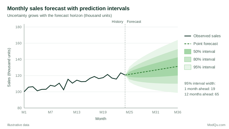
In Figure 1, the interval twelve months ahead is about 3.5 times as wide as the interval one month ahead, roughly in line with the square root of the horizon. Chatfield (1993) showed that published interval forecasts are frequently too narrow, partly because they ignore uncertainty about the model itself and partly because they assume the future will behave like the past. Checking intervals against outcomes is the remedy: if 95% intervals capture only 80% of actual results, they are overconfident. Good probabilistic forecasts should be both calibrated and as sharp as possible, and proper scoring rules reward exactly that combination (Gneiting et al., 2007).
Uncertainty in models
Many business figures come from models that combine several uncertain inputs. Market size, for example, is often estimated as the number of households × purchase intention × conversion rate × average spend. Errors in each input propagate into the output, and they do not simply add.
Monte Carlo simulation is the most practical way to propagate input uncertainty (Morgan & Henrion, 1990). Each input is given a probability distribution, the model is run many thousands of times with random draws, and the distribution of outputs is summarised. Consider a hypothetical market of 2.0 million households, with purchase intention of 34% (standard error 2.1 points, allowing for the design effect), an uncertain conversion from intention to purchase anywhere between 30% and 50%, and average spend of $120 (standard error $6). The point estimate is $32.6 million. In 200,000 simulated runs, the 90% interval is about $24.4 million to $41.7 million.
The simulation also shows which inputs matter most. Varying one input at a time while holding the others at their central values, the uncertain conversion rate alone produces about 77% of the full output variance, purchase intention for about 14% and spend for about 9%. This is a simple form of variance-based sensitivity analysis (Saltelli et al., 2008), and it points to an obvious action: research to pin down conversion is worth far more than a larger intention survey.
Model uncertainty needs separate treatment. Picking one model after trying many and reporting its intervals as if it had been chosen in advance understates uncertainty (Draper, 1995). Options include reporting results from several credible models side by side, averaging across models with weights that reflect their support (Hoeting et al., 1999), and validating on data not used to choose the model.
Communicating uncertainty
Uncertainty analysis only helps if decision-makers understand it. Research on communication suggests that stating uncertainty, numerically and plainly, does not generally reduce trust in the source (van der Bles et al., 2019). Useful practices include:
- Give a range alongside the central estimate, and say what the range covers: "sampling error only" is different from "all quantified sources".
- Use visual formats such as fan charts and interval plots rather than tables of standard errors.
- Separate quantified uncertainty from unquantified caveats, and list the second explicitly.
- Avoid false precision. Reporting market size as $32,640,000 implies knowledge nobody has.
Manski (2015) argues that official statistics are often presented as if they were exact, and that users would be better served by routine reporting of sampling and non-sampling uncertainty. The same applies to commercial reports.
Common mistakes
- Treating the margin of error as the total error. It covers sampling variability only, under the assumption of an unbiased design.
- Ignoring the design effect. Weighted and clustered samples are usually less precise than their nominal size suggests.
- Reporting forecasts without intervals, or with intervals that have never been checked against outcomes.
- Double counting or omitting correlations. If two inputs tend to move together, independent simulation draws misstate the output range.
- Hiding the assumptions. An interval is only as good as the distributions and models behind it.
Key takeaways
Uncertainty analysis asks three questions of any estimate, forecast or model: where could the error come from, how large could it be, and which sources matter most for the decision? Standard errors, design effects and the bootstrap handle sampling uncertainty; prediction intervals and calibration checks handle forecasts; Monte Carlo simulation and sensitivity analysis handle models with uncertain inputs. Reported clearly, uncertainty is not a weakness of the analysis but one of its most useful outputs.
References
Chatfield, C. (1993). Calculating interval forecasts. Journal of Business & Economic Statistics, 11(2), 121–135. https://doi.org/10.1080/07350015.1993.10509938
Der Kiureghian, A., & Ditlevsen, O. (2009). Aleatory or epistemic? Does it matter? Structural Safety, 31(2), 105–112. https://doi.org/10.1016/j.strusafe.2008.06.020
Draper, D. (1995). Assessment and propagation of model uncertainty. Journal of the Royal Statistical Society Series B: Statistical Methodology, 57(1), 45–97. https://doi.org/10.1111/j.2517-6161.1995.tb02015.x
Efron, B. (1979). Bootstrap methods: Another look at the jackknife. The Annals of Statistics, 7(1), 1–26. https://doi.org/10.1214/aos/1176344552
Efron, B., & Tibshirani, R. J. (1993). An introduction to the bootstrap. Chapman & Hall. https://doi.org/10.1007/978-1-4899-4541-9
Gneiting, T., Balabdaoui, F., & Raftery, A. E. (2007). Probabilistic forecasts, calibration and sharpness. Journal of the Royal Statistical Society Series B: Statistical Methodology, 69(2), 243–268. https://doi.org/10.1111/j.1467-9868.2007.00587.x
Groves, R. M., & Lyberg, L. (2010). Total survey error: Past, present, and future. Public Opinion Quarterly, 74(5), 849–879. https://doi.org/10.1093/poq/nfq065
Hoeting, J. A., Madigan, D., Raftery, A. E., & Volinsky, C. T. (1999). Bayesian model averaging: A tutorial. Statistical Science, 14(4), 382–417. https://doi.org/10.1214/ss/1009212519
Hyndman, R. J., & Athanasopoulos, G. (2021). Forecasting: Principles and practice (3rd ed.). OTexts.
Joint Committee for Guides in Metrology. (2008). Evaluation of measurement data: Guide to the expression of uncertainty in measurement (JCGM 100:2008). Bureau International des Poids et Mesures.
Kish, L. (1965). Survey sampling. Wiley.
Knight, F. H. (1921). Risk, uncertainty and profit. Houghton Mifflin.
Manski, C. F. (2015). Communicating uncertainty in official economic statistics: An appraisal fifty years after Morgenstern. Journal of Economic Literature, 53(3), 631–653. https://doi.org/10.1257/jel.53.3.631
Morgan, M. G., & Henrion, M. (1990). Uncertainty: A guide to dealing with uncertainty in quantitative risk and policy analysis. Cambridge University Press. https://doi.org/10.1017/CBO9780511840609
Rubin, D. B. (1987). Multiple imputation for nonresponse in surveys. Wiley. https://doi.org/10.1002/9780470316696
Saltelli, A., Ratto, M., Andres, T., Campolongo, F., Cariboni, J., Gatelli, D., Saisana, M., & Tarantola, S. (2008). Global sensitivity analysis: The primer. Wiley. https://doi.org/10.1002/9780470725184
van der Bles, A. M., van der Linden, S., Freeman, A. L. J., Mitchell, J., Galvão, A. B., Zaval, L., & Spiegelhalter, D. J. (2019). Communicating uncertainty about facts, numbers and science. Royal Society Open Science, 6(5), Article 181870. https://doi.org/10.1098/rsos.181870
Wolter, K. M. (2007). Introduction to variance estimation (2nd ed.). Springer. https://doi.org/10.1007/978-0-387-35099-8