
Statistics · Inference
Robustness Checks and Sensitivity Analyses in Strengthening Knowledge Claims
How robustness checks, specification curves and sensitivity analyses show whether a finding survives reasonable changes to the analysis, with a worked loyalty-programme example and practical guidance for business data.
Every statistical result depends on choices the analyst made along the way: which observations to keep, which variables to control for, how to treat outliers, whether to weight. Most of these choices are reasonable, and several alternatives are usually just as reasonable. A finding that holds only under one particular combination of choices is fragile. A finding that holds across many of them is much more credible. Robustness checks and sensitivity analyses are the tools for telling the two apart, and they are among the most effective ways to strengthen a knowledge claim before anyone acts on it.
Two related ideas
The terms are often used interchangeably, but it helps to separate them.
- A robustness check re-estimates the result under alternative, defensible analytic choices and asks whether the conclusion changes. Examples include adding or removing control variables, using a different outlier rule or re-running the analysis on a subsample.
- A sensitivity analysis asks how far an untestable assumption would have to be violated before the conclusion changed. The classic case is an unmeasured confounder: no dataset can rule it out, but analysts can calculate how strong it would need to be.
Lu and White (2014) point out that informal robustness checks are often run without a clear standard for what counts as "passing". A useful discipline is to state, before running each check, what result would weaken the claim.
Why single analyses mislead
Leamer (1983) famously argued that econometric results were believed far too readily because readers saw only the one specification the author chose to publish. Three decades later, Simmons et al. (2011) showed that undisclosed flexibility in data collection and analysis, such as choosing covariates or stopping rules after seeing the data, can push false-positive rates far above the nominal 5%. Gelman and Loken (2014) added that the problem does not require deliberate fishing: when analytic decisions depend on the data, a "garden of forking paths" produces apparently significant findings even when each analyst runs only one test.
Business analytics is just as exposed. A campaign evaluation, a driver analysis of satisfaction or a churn model may involve dozens of judgement calls. Robustness checks make those calls visible and show whether the headline result depends on them.
Standard robustness checks
Useful checks for survey and business data include:
- Alternative control sets. Does the estimated effect survive the addition of plausible confounders, such as prior spending or customer tenure?
- Outlier treatment. Do results change if extreme values are trimmed, winsorised or analysed with methods designed to resist them (Huber & Ronchetti, 2009)?
- Standard errors. Are conclusions the same with heteroskedasticity-consistent standard errors (White, 1980) or with clustering by store, region or interviewer?
- Weighting. Do weighted and unweighted estimates tell the same story? A large gap is itself informative about who the sample over- or under-represents.
- Subsamples and time periods. Does the effect hold for new and established customers, or before and after a price change?
- Alternative measures. Is the result specific to one wording of a question, or does it hold for a related measure of the same concept?
- Missing data. Do results hold under complete-case analysis, multiple imputation and plausible departures from the missing-at-random assumption (Little & Rubin, 2019)?
Mapping the whole space: specification curves
Running a handful of checks still leaves the reader to trust that the analyst picked the important ones. Two related methods address this by estimating the result under every reasonable combination of choices. Multiverse analysis reports the result across all defensible ways of constructing the dataset (Steegen et al., 2016). Specification curve analysis does the same for analytic choices and displays the estimates, sorted, alongside a panel showing which choices produced each one (Simonsohn et al., 2020). Young and Holsteen (2017) propose a similar multimodel framework that summarises how much of the variation in estimates comes from each modelling decision.
Consider a hypothetical analysis of whether loyalty programme members spend more per year than non-members. Four choices each have defensible options: the control variables (none, demographics, demographics plus past spend, or a full set), the outlier rule (keep, trim the top 1% or winsorise), whether to apply survey weights, and whether to restrict the sample to active customers. That gives 4 × 3 × 2 × 2 = 48 specifications.
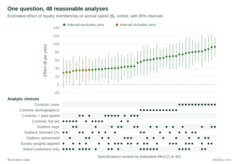
A report that showed only the specification with demographic controls and no other adjustments would claim an effect of about $69 per year (95% interval $46 to $93). Figure 1 tells a more nuanced story. The direction of the effect is robust: all 48 estimates are positive, and 44 of the 48 intervals exclude zero. The size is not. The median estimate is about $81 without controls but falls to about $41 once past spend is included, because customers who already spent more were more likely to join. The honest conclusion is "members spend more, probably by $30 to $45 a year after allowing for prior behaviour", not "the programme adds $69".
Sensitivity to unmeasured confounding
Observational data can never rule out a confounder that was not measured. Sensitivity analysis turns that worry into a number. The idea goes back to Cornfield et al. (1959), who showed that for a hidden factor to explain away the association between smoking and lung cancer, it would have to be far more strongly related to smoking than any plausible candidate. Rosenbaum (2002) formalised the approach for matched observational studies.
A simple modern version is the E-value (VanderWeele & Ding, 2017). For an observed risk ratio RR above 1:
E-value = RR + √( RR × (RR − 1) )
Suppose a hypothetical customer survey finds that people who used a self-service portal were 1.8 times as likely to renew, with a lower 95% confidence limit of 1.3. The E-value is 1.8 + √(1.8 × 0.8) = 3.0. An unmeasured confounder would need to be associated with both portal use and renewal by a risk ratio of at least 3.0 each to explain the association away; to move the confidence interval to include 1, a risk ratio of about 1.9 would suffice. Whether such a confounder is plausible is a substantive judgement, but the analysis makes that judgement explicit.
For regression models, related tools ask how much the estimate would change if unobserved variables were as important as the observed controls. Altonji et al. (2005) introduced this idea, Oster (2019) linked it to how coefficients and R² move as controls are added, and Cinelli and Hazlett (2020) expressed it in terms of partial R² values that can be benchmarked against observed covariates.
Sensitivity to missing data
Surveys almost always have missing answers, and standard methods such as multiple imputation assume that values are missing at random given the observed variables. That assumption cannot be tested from the data. A practical sensitivity analysis, sometimes called delta adjustment, imputes the missing values under the standard assumption and then shifts them by a series of fixed amounts, for example assuming that nonrespondents to a satisfaction question score 0.5, 1 or 2 points lower than similar respondents (Little & Rubin, 2019). If the conclusion survives every shift that subject experts consider plausible, it does not depend on the missing-at-random assumption. If it reverses at a small shift, the report should say so.
Practical guidance
- Plan the checks in advance. Listing intended robustness checks in an analysis plan, or a formal pre-registration, prevents the temptation to report only the ones that pass (Nosek et al., 2018).
- Choose checks that could break the claim. A check that cannot change the conclusion adds length, not credibility. Target the assumptions most likely to be wrong.
- Report everything you ran, including checks where the result weakened, ideally in an appendix or a specification curve.
- Distinguish direction from size. As in the loyalty example, a result can be robust in sign while its magnitude depends heavily on choices.
- Summarise robustness in plain language. Decision-makers rarely need every specification. A sentence such as "the effect was positive in all 48 analyses; its size ranged from $29 to $93, depending mainly on whether prior spending was controlled" is often enough.
- Look for independent lines of evidence. No amount of re-analysis of one dataset removes biases shared by all specifications. Triangulating across designs and data sources with different weaknesses is stronger still (Lawlor et al., 2016; Munafò & Davey Smith, 2018).
Common mistakes
- Treating robustness checks as a ritual. Adding a table of near-identical models signals diligence without testing anything important.
- Equating robustness with truth. If every specification shares the same biased sample or the same flawed measure, the results will agree and still be wrong.
- Defining "robust" as "significant everywhere". Intervals that move from just above to just below the threshold are not evidence of fragility; large changes in the estimate are.
- Including unreasonable specifications. A specification curve should contain only choices a competent analyst could defend, or it will understate robustness.
- Forgetting the decision. The relevant question is whether a different analysis would lead to a different business decision, not whether a coefficient changes in the second decimal place.
Key takeaways
A knowledge claim is only as strong as its weakest unexamined assumption. Robustness checks test whether a result survives reasonable alternative analyses; sensitivity analyses quantify how wrong an untestable assumption would have to be to overturn it. Specification curves and multiverse analyses show the full range of defensible answers, and tools such as the E-value put unmeasured confounding on a numerical scale. Used honestly, with checks chosen to challenge the claim and all results reported, these methods turn a single fragile estimate into evidence that decision-makers can trust.
References
Altonji, J. G., Elder, T. E., & Taber, C. R. (2005). Selection on observed and unobserved variables: Assessing the effectiveness of Catholic schools. Journal of Political Economy, 113(1), 151–184. https://doi.org/10.1086/426036
Cinelli, C., & Hazlett, C. (2020). Making sense of sensitivity: Extending omitted variable bias. Journal of the Royal Statistical Society Series B: Statistical Methodology, 82(1), 39–67. https://doi.org/10.1111/rssb.12348
Cornfield, J., Haenszel, W., Hammond, E. C., Lilienfeld, A. M., Shimkin, M. B., & Wynder, E. L. (1959). Smoking and lung cancer: Recent evidence and a discussion of some questions. Journal of the National Cancer Institute, 22(1), 173–203. https://doi.org/10.1093/jnci/22.1.173
Gelman, A., & Loken, E. (2014). The statistical crisis in science. American Scientist, 102(6), 460–465. https://doi.org/10.1511/2014.111.460
Huber, P. J., & Ronchetti, E. M. (2009). Robust statistics (2nd ed.). Wiley. https://doi.org/10.1002/9780470434697
Lawlor, D. A., Tilling, K., & Davey Smith, G. (2016). Triangulation in aetiological epidemiology. International Journal of Epidemiology, 45(6), 1866–1886. https://doi.org/10.1093/ije/dyw314
Leamer, E. E. (1983). Let's take the con out of econometrics. The American Economic Review, 73(1), 31–43.
Little, R. J. A., & Rubin, D. B. (2019). Statistical analysis with missing data (3rd ed.). Wiley. https://doi.org/10.1002/9781119482260
Lu, X., & White, H. (2014). Robustness checks and robustness tests in applied economics. Journal of Econometrics, 178(Part 1), 194–206. https://doi.org/10.1016/j.jeconom.2013.08.016
Munafò, M. R., & Davey Smith, G. (2018). Robust research needs many lines of evidence. Nature, 553(7689), 399–401. https://doi.org/10.1038/d41586-018-01023-3
Nosek, B. A., Ebersole, C. R., DeHaven, A. C., & Mellor, D. T. (2018). The preregistration revolution. Proceedings of the National Academy of Sciences, 115(11), 2600–2606. https://doi.org/10.1073/pnas.1708274114
Oster, E. (2019). Unobservable selection and coefficient stability: Theory and evidence. Journal of Business & Economic Statistics, 37(2), 187–204. https://doi.org/10.1080/07350015.2016.1227711
Rosenbaum, P. R. (2002). Observational studies (2nd ed.). Springer. https://doi.org/10.1007/978-1-4757-3692-2
Simmons, J. P., Nelson, L. D., & Simonsohn, U. (2011). False-positive psychology: Undisclosed flexibility in data collection and analysis allows presenting anything as significant. Psychological Science, 22(11), 1359–1366. https://doi.org/10.1177/0956797611417632
Simonsohn, U., Simmons, J. P., & Nelson, L. D. (2020). Specification curve analysis. Nature Human Behaviour, 4(11), 1208–1214. https://doi.org/10.1038/s41562-020-0912-z
Steegen, S., Tuerlinckx, F., Gelman, A., & Vanpaemel, W. (2016). Increasing transparency through a multiverse analysis. Perspectives on Psychological Science, 11(5), 702–712. https://doi.org/10.1177/1745691616658637
VanderWeele, T. J., & Ding, P. (2017). Sensitivity analysis in observational research: Introducing the E-value. Annals of Internal Medicine, 167(4), 268–274. https://doi.org/10.7326/M16-2607
White, H. (1980). A heteroskedasticity-consistent covariance matrix estimator and a direct test for heteroskedasticity. Econometrica, 48(4), 817–838. https://doi.org/10.2307/1912934
Young, C., & Holsteen, K. (2017). Model uncertainty and robustness: A computational framework for multimodel analysis. Sociological Methods & Research, 46(1), 3–40. https://doi.org/10.1177/0049124115610347