
Statistics · Data science and machine learning
Transfer Learning Approaches in Statistical Modeling
How transfer learning uses data or models from a related setting to build better models where local data are scarce, which statistical forms it takes, and how to avoid transfer that makes results worse.
A company that has run customer surveys in its home market for ten years plans to enter a new country. It has thousands of past responses at home and only a few hundred from a pilot study abroad. A model built only on the pilot data will be noisy; a model built only on home data may not fit the new market. Transfer learning is the set of methods that use knowledge from a related source setting to improve learning in a target setting where data are limited (Pan & Yang, 2010).
The idea is old in statistics, even if the name comes from machine learning. Whenever an analyst uses a previous study to set a prior, pools data across regions or borrows strength from related groups, knowledge is being transferred. What has changed is the scale: modern models trained on enormous data sets are routinely adapted to new tasks with modest data.
When is transfer possible?
Transfer works when source and target share structure. Pan and Yang (2010) distinguish two broad differences that can separate them. The domain may differ: the inputs come from a different population, such as younger customers or a different country. The task may differ: the outcome or the relationship between inputs and outcome changes, such as predicting churn instead of satisfaction.
Statistical work on dataset shift classifies the domain differences more finely (Moreno-Torres et al., 2012). Under covariate shift, the distribution of inputs changes but the relationship between inputs and outcome stays the same. Under prior probability shift, the share of each outcome class changes. Under concept shift, the relationship itself changes. Each type calls for a different response, and concept shift is the hardest to deal with because the source model is partly wrong for the target.
Main approaches
Reweighting. Under covariate shift, source observations can be given weights proportional to how common their inputs are in the target relative to the source. Shimodaira (2000) showed that weighting the likelihood in this way improves prediction for the target population. Survey researchers will recognise the idea: it is closely related to weighting a sample to match a population.
Shrinking towards the source. A target model can be estimated with a penalty that pulls its coefficients towards those of the source model, rather than towards zero. If the target data strongly disagree with the source, the estimates move away; if the data are thin, the estimates stay close to the source. This is the logic of multilevel models, in which each group's estimate is pulled towards the overall mean by an amount that depends on the group's sample size (Gelman & Hill, 2007). Recent statistical work makes it precise for high-dimensional regression: Bastani (2021) uses a large proxy data set to estimate most of a model and corrects it with a sparse adjustment from a small gold-standard data set, while Li et al. (2022) and Tian and Feng (2023) develop methods that also detect which of several source data sets are useful.
Feature transfer and fine-tuning. In deep learning, a network trained on a large source data set learns general features, such as edges in images or word meanings in text (LeCun et al., 2015). These features can be reused for a new task by keeping the early layers and retraining the final ones, or by continuing training on the target data with a small learning rate, called fine-tuning. Pretrained language models such as BERT (Devlin et al., 2019) made this the standard approach for text classification, including the coding of open-ended survey responses. Weiss et al. (2016) and Zhuang et al. (2021) survey the many variants.
A worked example
Figure 1 shows a simulation of the market-entry problem. A linear model with 30 predictors of customer spending is well estimated from 5,000 observations in the home market. In the new market, the true coefficients differ slightly from those at home. Three approaches are compared on how accurately they predict spending in the new market.
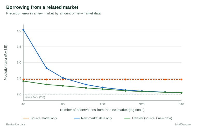
Using the home model unchanged gives an error of 2.47, which never improves because it ignores local data. A model fitted only to new-market data is very poor with 40 observations (error 4.03) and needs about 80 observations to match the home model. The transfer model, which starts from the home coefficients and adjusts them with a penalty chosen by cross-validation, is better than both at every sample size: with 40 local observations its error is 2.42, and with 120 it is 2.20, against 2.31 for the local-only model. As local data grow, the two approaches converge, because the local data become sufficient on their own. In practice, transfer is most valuable at exactly the point where a business has to decide on a new market with little information.
Uses in survey and market research
Transfer learning fits several routine problems in survey work. A satisfaction driver model built for one brand can serve as the starting point for a sister brand with a smaller customer base. A classifier that codes open-ended answers in one language can be adapted to another with a few hundred hand-coded examples. Estimates for small regions or rare customer segments can borrow from larger ones, as in small area estimation. A model of response propensity from past survey waves can guide fieldwork in a new wave before its own data arrive. In each case, the source supplies the structure and the target data adjust it.
Negative transfer and other risks
Transfer can also make things worse. Negative transfer occurs when the source is too different from the target, so that borrowing from it introduces bias that outweighs the gain in precision (Wang et al., 2019). The risk is greatest when the analyst assumes similarity without testing it. Ben-David et al. (2010) showed that how well a model transfers depends on how well it fits the source and on how different the two input distributions are, which can be measured from data.
Other risks include hidden differences in measurement, such as survey questions that are translated differently or rating scales that are used differently across cultures, and source bias that carries over to the target, such as unfair patterns learned by a pretrained language model.
Practical guidance
- Check similarity first. Compare the input distributions and, where possible, fit both models on a small target sample to see how far the coefficients differ.
- Let the data decide how much to borrow. Use cross-validation or a multilevel structure to set the amount of shrinkage towards the source, rather than fixing it in advance.
- Always compare with a target-only baseline. If transfer does not beat it on held-out target data, do not use it.
- Harmonise measurement. Make sure that variables mean the same thing in both settings before pooling.
- Monitor after deployment. As target data accumulate, re-estimate and reduce reliance on the source.
Key takeaways
Transfer learning uses knowledge from a related setting to build better models where data are scarce. In statistics it appears as reweighting, shrinkage towards a source model and multilevel pooling; in machine learning as reusing and fine-tuning pretrained models. It helps most when target data are limited and the source is genuinely similar, and it can harm results when that similarity is assumed rather than checked. Used with a target-only baseline and data-driven control of how much to borrow, it lets researchers produce useful knowledge from the first small samples in a new market, population or task.
References
Bastani, H. (2021). Predicting with proxies: Transfer learning in high dimension. Management Science, 67(5), 2964–2984. https://doi.org/10.1287/mnsc.2020.3729
Ben-David, S., Blitzer, J., Crammer, K., Kulesza, A., Pereira, F., & Vaughan, J. W. (2010). A theory of learning from different domains. Machine Learning, 79(1–2), 151–175. https://doi.org/10.1007/s10994-009-5152-4
Devlin, J., Chang, M.-W., Lee, K., & Toutanova, K. (2019). BERT: Pre-training of deep bidirectional transformers for language understanding. In Proceedings of the 2019 Conference of the North American Chapter of the Association for Computational Linguistics: Human Language Technologies, Volume 1 (Long and Short Papers) (pp. 4171–4186). Association for Computational Linguistics. https://doi.org/10.18653/v1/N19-1423
Gelman, A., & Hill, J. (2007). Data analysis using regression and multilevel/hierarchical models. Cambridge University Press. https://doi.org/10.1017/CBO9780511790942
LeCun, Y., Bengio, Y., & Hinton, G. (2015). Deep learning. Nature, 521(7553), 436–444. https://doi.org/10.1038/nature14539
Li, S., Cai, T. T., & Li, H. (2022). Transfer learning for high-dimensional linear regression: Prediction, estimation and minimax optimality. Journal of the Royal Statistical Society Series B: Statistical Methodology, 84(1), 149–173. https://doi.org/10.1111/rssb.12479
Moreno-Torres, J. G., Raeder, T., Alaiz-Rodríguez, R., Chawla, N. V., & Herrera, F. (2012). A unifying view on dataset shift in classification. Pattern Recognition, 45(1), 521–530. https://doi.org/10.1016/j.patcog.2011.06.019
Pan, S. J., & Yang, Q. (2010). A survey on transfer learning. IEEE Transactions on Knowledge and Data Engineering, 22(10), 1345–1359. https://doi.org/10.1109/TKDE.2009.191
Shimodaira, H. (2000). Improving predictive inference under covariate shift by weighting the log-likelihood function. Journal of Statistical Planning and Inference, 90(2), 227–244. https://doi.org/10.1016/S0378-3758(00)00115-4
Tian, Y., & Feng, Y. (2023). Transfer learning under high-dimensional generalized linear models. Journal of the American Statistical Association, 118(544), 2684–2697. https://doi.org/10.1080/01621459.2022.2071278
Wang, Z., Dai, Z., Póczos, B., & Carbonell, J. (2019). Characterizing and avoiding negative transfer. In Proceedings of the IEEE/CVF Conference on Computer Vision and Pattern Recognition (pp. 11285–11294). IEEE. https://doi.org/10.1109/CVPR.2019.01155
Weiss, K., Khoshgoftaar, T. M., & Wang, D. (2016). A survey of transfer learning. Journal of Big Data, 3, Article 9. https://doi.org/10.1186/s40537-016-0043-6
Zhuang, F., Qi, Z., Duan, K., Xi, D., Zhu, Y., Zhu, H., Xiong, H., & He, Q. (2021). A comprehensive survey on transfer learning. Proceedings of the IEEE, 109(1), 43–76. https://doi.org/10.1109/JPROC.2020.3004555