
Statistics · Tests and models
The t-Test: Comparing Two Means
How the t-test compares two averages, when to use the one-sample, paired, Student and Welch versions, a worked advertising example, and how to report effect sizes and intervals rather than p-values alone.
Is the average satisfaction score higher in one region than another? Did a new advertising concept raise purchase intention compared with the old one? Do customers spend more after a website redesign? Each of these questions compares two averages, and the most common tool for answering them is the t-test. It is simple, well understood and available in every statistics package, but it is also easy to misuse. This article explains how the test works, which version to choose, how to read and report the result, and where its limits lie.
A brewer's problem
The t-test was published in 1908 by William Sealy Gosset, a chemist at the Guinness brewery in Dublin, writing under the pseudonym "Student" (Student, 1908). Gosset worked with very small samples of barley and hops, and he noticed that the usual normal-distribution methods gave intervals that were too narrow when the standard deviation had to be estimated from only a few observations. His solution was a new distribution that allowed for the extra uncertainty. Zabell (2008) gives an accessible account of the paper and its context. Fisher (1925) later recast the statistic in its modern form and made it a standard method through his widely read textbook.
The logic of the test
Every t-test has the same structure. It divides a difference by its standard error:
t = (observed difference − difference under H0) ÷ standard error of the difference
The numerator is the signal: how far the observed difference is from what the null hypothesis expects, usually zero. The denominator is the noise: how much the difference would vary from sample to sample by chance alone. A t value near 0 means the difference is small relative to that noise; a large positive or negative value means it is unusually large if the null hypothesis were true.
If the data are drawn from normal populations, the statistic follows a t distribution under the null hypothesis. The t distribution looks like the normal curve but has heavier tails, and its exact shape depends on the degrees of freedom, which grow with the sample size. With few degrees of freedom, larger t values are needed to reach the same level of statistical significance. As the degrees of freedom rise, the t distribution approaches the normal.
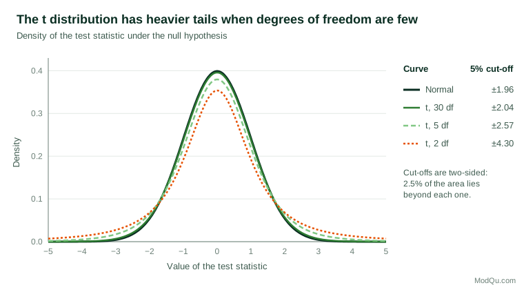
The p-value is the probability, under the null hypothesis, of a t value at least as extreme as the one observed. A confidence interval for the difference is built from the same ingredients: the observed difference plus or minus a critical t value times the standard error.
Three kinds of t-test
One-sample t-test
The one-sample test compares a sample mean with a fixed reference value. A brand might ask whether average satisfaction differs from an industry benchmark of 7.0, or whether average order value differs from a target. The standard error is s ÷ √n, where s is the sample standard deviation, and the degrees of freedom are n − 1.
Paired t-test
The paired test is used when each observation in one group is matched to one in the other: the same respondents rate two packaging designs, or the same stores are measured before and after a promotion. The test works on the differences within each pair, which turns it into a one-sample test of whether the mean difference is zero. Pairing removes stable differences between individuals and is often far more powerful than comparing independent groups of the same size.
Independent two-sample t-test
The independent test compares two separate groups, such as customers who saw concept A and customers who saw concept B. There are two versions. Student's original version pools the two sample variances, assuming the populations have the same variance. Welch (1947) proposed a version that does not make that assumption. Its standard error is:
SE = √( s12 ÷ n1 + s22 ÷ n2 )
and its degrees of freedom are approximated with the Welch–Satterthwaite formula (Satterthwaite, 1946):
df ≈ (s12/n1 + s22/n2)2 ÷ [ (s12/n1)2/(n1 − 1) + (s22/n2)2/(n2 − 1) ]
When variances and group sizes are equal the two versions give almost identical answers. When they differ, especially when the smaller group has the larger variance, Student's version can produce far too many false positives, while Welch's test keeps close to its nominal error rate. For that reason, several methodologists recommend Welch's test as the default for independent groups (Delacre et al., 2017; Ruxton, 2006). Running a preliminary test of equal variances and then choosing between the two versions is not a good alternative: the two-step procedure distorts the overall error rate (Zimmerman, 2004).
A worked example
Suppose a hypothetical concept test shows one of two advertisements to separate random samples of respondents, who then rate purchase intention on a 0 to 10 scale. The summary results are:
| Group | n | Mean | Standard deviation |
|---|---|---|---|
| Concept A | 120 | 6.4 | 1.8 |
| Concept B | 95 | 5.8 | 2.4 |
The observed difference is 0.6 points. Using Welch's formula, the standard error is √(1.8² ÷ 120 + 2.4² ÷ 95) ≈ 0.296, so t ≈ 0.6 ÷ 0.296 ≈ 2.03, with about 170 degrees of freedom. The two-sided p-value is 0.044, and the 95% confidence interval for the difference runs from 0.02 to 1.18 points.
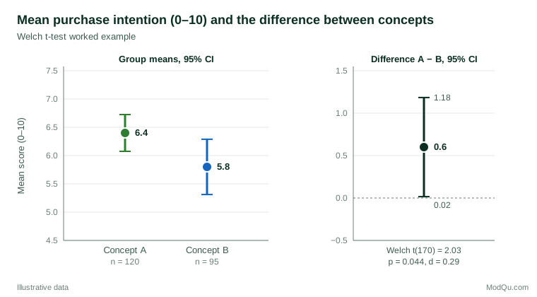
Three points stand out. First, the result is statistically significant at the 5% level, but only just; the interval for the difference stretches from almost nothing to more than a point. Second, the individual confidence intervals in Figure 2 overlap, yet the difference is significant. Overlapping intervals do not imply a non-significant difference, a common misreading that the separate interval for the difference avoids (Cumming, 2014). Third, Student's pooled test on the same data gives t = 2.09 and p = 0.037. The gap is small here, but it grows when group sizes and variances are more unequal.
Effect size: how big is the difference?
A p-value says whether a difference is distinguishable from zero, not whether it matters. An effect size expresses the size of the difference on a standard scale. The most common for two means is Cohen's d: the difference divided by the pooled standard deviation (Cohen, 1988).
d = (x̄1 − x̄2) ÷ spooled
In the example, the pooled standard deviation is about 2.09, so d ≈ 0.6 ÷ 2.09 ≈ 0.29. Hedges (1981) showed that d slightly overstates the population value in small samples and proposed a correction, now known as Hedges' g; with 215 respondents the corrected value is still 0.29. Cohen (1988) suggested 0.2, 0.5 and 0.8 as rough markers of small, medium and large effects, but he intended them as a last resort. In business settings the raw difference in meaningful units, such as 0.6 points on the purchase-intention scale or $4 of average spend, is usually more useful. Lakens (2013) gives a practical guide to calculating and reporting effect sizes for t-tests, including the different versions for paired designs.
A paired example
Suppose 40 hypothetical respondents rate both the current and a redesigned package on the same 0 to 10 scale. The mean difference (new minus current) is 0.45 points, and the standard deviation of the differences is 1.2. The standard error is 1.2 ÷ √40 ≈ 0.19, so t(39) ≈ 2.37, p ≈ 0.023, and the 95% confidence interval for the mean difference is 0.07 to 0.83 points. Had the same ratings been analysed as two independent groups, the large differences between individual respondents would have inflated the standard error, and the result might not have been significant. Choosing the test that matches the design is not a technicality; it determines how much the data can show.
Assumptions and how much they matter
Independence. Observations must be independent within and between groups (except for the deliberate pairing in a paired test). This is the assumption that matters most. Repeated responses from the same person, clustered samples and panel data all violate it, and standard t-tests then understate the standard error.
Normality. The test assumes normally distributed populations, but thanks to the central limit theorem the sampling distribution of a mean becomes close to normal as the sample grows. Lumley et al. (2002) showed that in large samples the t-test remains valid even for strongly skewed outcomes such as health costs. With small samples and heavy skew or extreme outliers, it is less reliable.
Equal variances. Required only for Student's pooled version, and avoided altogether by using Welch's test.
Measurement scale. Survey ratings are ordinal, but means of rating scales with five or more points are widely and usually reasonably analysed with t-tests, especially when samples are moderate in size.
When assumptions are doubtful, alternatives exist. The Wilcoxon signed-rank test (Wilcoxon, 1945) and the Wilcoxon–Mann–Whitney rank-sum test (Mann & Whitney, 1947) compare groups using ranks rather than raw values. They answer a slightly different question, however: they test whether values in one group tend to be larger than in the other, not whether the means differ. Fagerland (2012) shows that in large samples the rank tests can reject when the means are equal but the distributions differ in shape, and argues that the t-test is often the better choice when the mean is the quantity of interest. Bootstrap confidence intervals are a further option for skewed data.
The t-test in survey and business practice
Weighted and complex samples. Textbook formulas assume simple random sampling. Survey weights, stratification and clustering change the standard error, and the design effect can make a "significant" unweighted result non-significant once the design is respected (Kish, 1965). Survey software estimates design-based standard errors and degrees of freedom for comparisons of means (Lumley, 2010).
A/B tests. Online experiments typically compare mean revenue, time on site or conversion between two randomly assigned groups, and the Welch t-test is the workhorse of such comparisons. Kohavi et al. (2020) describe practical issues including heavily skewed revenue metrics, the need to analyse at the level at which units were randomised, and the danger of stopping a test as soon as the p-value dips below 0.05.
Many comparisons. A tracking study that runs t-tests on 40 attributes across six segments will produce several "significant" differences by chance alone. Controlling the false discovery rate is a practical remedy when many comparisons are made (Benjamini & Hochberg, 1995).
Planning sample size. Small effects require large samples. To detect a difference of d = 0.25 with 80% power in a two-sided test at the 5% level, a study needs about 253 respondents per group (Cohen, 1988). Running an underpowered test and concluding "no difference" is one of the most common errors in applied work.
Showing that groups are similar. A non-significant t-test does not show that two means are equal. When the goal is to demonstrate similarity, for example that a cheaper ingredient does not reduce taste ratings, an equivalence test is needed. The two one-sided tests (TOST) procedure asks whether the difference is reliably inside a pre-specified margin (Schuirmann, 1987), and Lakens (2017) gives a practical introduction.
Reporting a t-test
A complete report includes the means and standard deviations of each group, the sample sizes, the version of the test, the t value with degrees of freedom, the p-value, the difference with its confidence interval and an effect size. For the worked example: "Purchase intention was higher for concept A (M = 6.4, SD = 1.8, n = 120) than for concept B (M = 5.8, SD = 2.4, n = 95), a difference of 0.6 points, 95% CI [0.02, 1.18]; Welch t(170) = 2.03, p = 0.044, d = 0.29." The American Statistical Association's statement on p-values stresses that a p-value alone does not measure the size or importance of an effect and should not be the sole basis of a decision (Wasserstein & Lazar, 2016).
Common mistakes
- Using an independent test on paired data, or a paired test on independent groups.
- Defaulting to Student's pooled test when group variances or sizes differ; Welch's test is the safer default.
- Reading overlapping confidence intervals as "no difference". Test or estimate the difference directly.
- Treating "not significant" as "no effect", especially in small samples.
- Ignoring survey weights and clustering, which usually makes results look more precise than they are.
- Running dozens of t-tests without adjustment and highlighting the few that cross the threshold.
- Reporting only the p-value, without the size of the difference or its uncertainty.
Key takeaways
The t-test compares a difference in means with the noise expected from sampling, and the t distribution accounts for the extra uncertainty of estimating that noise from the data. Use the paired test for matched observations and Welch's test as the default for independent groups. The test is robust to non-normality in moderate and large samples, but not to dependence between observations or to ignoring the survey design. Above all, report the difference, its confidence interval and an effect size alongside the p-value, so that decision-makers can judge whether the difference is large enough to matter.
References
Benjamini, Y., & Hochberg, Y. (1995). Controlling the false discovery rate: A practical and powerful approach to multiple testing. Journal of the Royal Statistical Society Series B: Statistical Methodology, 57(1), 289–300. https://doi.org/10.1111/j.2517-6161.1995.tb02031.x
Cohen, J. (1988). Statistical power analysis for the behavioral sciences (2nd ed.). Routledge. https://doi.org/10.4324/9780203771587
Cumming, G. (2014). The new statistics: Why and how. Psychological Science, 25(1), 7–29. https://doi.org/10.1177/0956797613504966
Delacre, M., Lakens, D., & Leys, C. (2017). Why psychologists should by default use Welch's t-test instead of Student's t-test. International Review of Social Psychology, 30(1), 92–101. https://doi.org/10.5334/irsp.82
Fagerland, M. W. (2012). t-tests, non-parametric tests, and large studies: A paradox of statistical practice? BMC Medical Research Methodology, 12, Article 78. https://doi.org/10.1186/1471-2288-12-78
Fisher, R. A. (1925). Statistical methods for research workers. Oliver and Boyd.
Hedges, L. V. (1981). Distribution theory for Glass's estimator of effect size and related estimators. Journal of Educational Statistics, 6(2), 107–128. https://doi.org/10.3102/10769986006002107
Kish, L. (1965). Survey sampling. Wiley.
Kohavi, R., Tang, D., & Xu, Y. (2020). Trustworthy online controlled experiments: A practical guide to A/B testing. Cambridge University Press. https://doi.org/10.1017/9781108653985
Lakens, D. (2013). Calculating and reporting effect sizes to facilitate cumulative science: A practical primer for t-tests and ANOVAs. Frontiers in Psychology, 4, Article 863. https://doi.org/10.3389/fpsyg.2013.00863
Lakens, D. (2017). Equivalence tests: A practical primer for t tests, correlations, and meta-analyses. Social Psychological and Personality Science, 8(4), 355–362. https://doi.org/10.1177/1948550617697177
Lumley, T. (2010). Complex surveys: A guide to analysis using R. Wiley. https://doi.org/10.1002/9780470580066
Lumley, T., Diehr, P., Emerson, S., & Chen, L. (2002). The importance of the normality assumption in large public health data sets. Annual Review of Public Health, 23(1), 151–169. https://doi.org/10.1146/annurev.publhealth.23.100901.140546
Mann, H. B., & Whitney, D. R. (1947). On a test of whether one of two random variables is stochastically larger than the other. The Annals of Mathematical Statistics, 18(1), 50–60. https://doi.org/10.1214/aoms/1177730491
Ruxton, G. D. (2006). The unequal variance t-test is an underused alternative to Student's t-test and the Mann–Whitney U test. Behavioral Ecology, 17(4), 688–690. https://doi.org/10.1093/beheco/ark016
Satterthwaite, F. E. (1946). An approximate distribution of estimates of variance components. Biometrics Bulletin, 2(6), 110–114. https://doi.org/10.2307/3002019
Schuirmann, D. J. (1987). A comparison of the two one-sided tests procedure and the power approach for assessing the equivalence of average bioavailability. Journal of Pharmacokinetics and Biopharmaceutics, 15(6), 657–680. https://doi.org/10.1007/BF01068419
Student. (1908). The probable error of a mean. Biometrika, 6(1), 1–25. https://doi.org/10.1093/biomet/6.1.1
Wasserstein, R. L., & Lazar, N. A. (2016). The ASA statement on p-values: Context, process, and purpose. The American Statistician, 70(2), 129–133. https://doi.org/10.1080/00031305.2016.1154108
Welch, B. L. (1947). The generalization of "Student's" problem when several different population variances are involved. Biometrika, 34(1–2), 28–35. https://doi.org/10.1093/biomet/34.1-2.28
Wilcoxon, F. (1945). Individual comparisons by ranking methods. Biometrics Bulletin, 1(6), 80–83. https://doi.org/10.2307/3001968
Zabell, S. L. (2008). On Student's 1908 article "The probable error of a mean". Journal of the American Statistical Association, 103(481), 1–7. https://doi.org/10.1198/016214508000000030
Zimmerman, D. W. (2004). A note on preliminary tests of equality of variances. British Journal of Mathematical and Statistical Psychology, 57(1), 173–181. https://doi.org/10.1348/000711004849222