
Statistics · Tests and models
Analysis of Variance (ANOVA) and Its Extensions
How analysis of variance compares the means of three or more groups, how to read the F ratio and effect sizes, and when to use Welch, factorial, repeated-measures and covariance extensions.
Market researchers often need to compare more than two groups at once. Do three packaging designs differ in willingness to pay? Does satisfaction vary across five regions? Running a separate t-test for every pair of groups inflates the chance of a false positive, because each extra test is another opportunity for a Type I error. Analysis of variance (ANOVA), developed by R. A. Fisher and set out for practitioners in his 1925 textbook (Fisher, 1925), answers the overall question with a single test: is there more variation between the group means than we would expect from the variation within the groups?
The logic of the F ratio
ANOVA splits the total variation in an outcome into two parts. The between-group part reflects how far each group mean lies from the grand mean. The within-group part reflects how far individual respondents lie from their own group mean, which is treated as noise. Each part is divided by its degrees of freedom to give a mean square, and the test statistic is their ratio:
F = MSbetween ÷ MSwithin
If the population means are all equal, F should be close to 1. A large F means the group means are further apart than within-group noise alone would explain. The null hypothesis is that all population means are equal; the alternative is that at least one differs. A significant F therefore says that some difference exists, not where it lies.
A worked example
Suppose a hypothetical concept test shows each of three packaging designs to 50 respondents and asks how much they would pay. The group means are $62, $68 and $74, and the standard deviation within each group is $20. The between-group sum of squares is 50 × (6² + 0² + 6²) = 3,600 on 2 degrees of freedom, so MSbetween = 1,800. The within-group mean square is 20² = 400 on 147 degrees of freedom. The result is F(2, 147) = 1,800 ÷ 400 = 4.5, with p = .013.
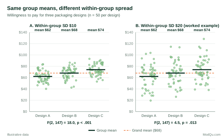
Figure 1 shows why the within-group spread matters. With the same means but half the spread, F rises to 18.0. Statistical significance is not the same as importance, so ANOVA results should always be reported with an effect size. Eta squared, the share of total variation explained by group membership, is 3,600 ÷ 62,400 = 0.058 here. Omega squared corrects its small upward bias and gives about 0.045. Lakens (2013) and Olejnik and Algina (2003) explain which version to report for different designs.
Assumptions and how robust ANOVA is
Classical ANOVA assumes independent observations, roughly normal residuals and equal variances across groups. An extensive review of earlier empirical studies by Glass et al. (1972) found the F test fairly robust to non-normality, but sensitive to unequal variances when group sizes also differ. Independence matters most of all: repeated answers from the same respondent, or clustered samples, break the test unless the design is modelled.
Unequal variances are common in business data. Welch (1951) proposed a version of the F test that does not assume equal variances, and Delacre et al. (2019) argue that Welch's F should be the default, since it loses little power when variances are equal and protects the error rate when they are not. Tests of equal variances, such as the median-based version of Levene's test studied by Brown and Forsythe (1974), are informative but should not act as a gatekeeper for choosing the main test.
Finding which groups differ
A significant overall F is usually followed by post hoc comparisons. Tukey's (1949) honestly significant difference procedure compares every pair of means while holding the familywise error rate at the chosen level. When variances or group sizes are unequal, the Games–Howell procedure is preferred (Games & Howell, 1976). For a small number of planned comparisons decided before seeing the data, specific contrasts are more powerful than testing every pair.
Extensions of the basic model
- Two-way and factorial ANOVA. Two or more factors, such as design and price point, are crossed. The model tests each main effect and their interaction: whether the effect of design depends on the price. Interactions often carry the most useful business insight.
- Repeated-measures ANOVA. The same respondents rate every concept, which removes stable individual differences from the error term and increases power. It adds a sphericity assumption; when this is doubtful, the degrees of freedom are reduced using the correction proposed by Greenhouse and Geisser (1959).
- Analysis of covariance (ANCOVA). A continuous covariate, such as prior spending, is added to reduce error variance or adjust for baseline differences. It works best in randomised designs and should not be expected to remove confounding in observational data.
- Multivariate ANOVA (MANOVA). Several related outcomes, such as liking, relevance and purchase intent, are tested together.
- Non-parametric alternatives. When outcomes are ranks or strongly skewed, the Kruskal–Wallis test compares groups using ranks.
All of these are special cases of the general linear model, which means they can also be fitted as a regression with dummy-coded groups.
Practical guidance for survey data
Weighted or clustered survey samples need design-based tests, because ordinary ANOVA assumes simple random sampling and understates standard errors when the design effect is large. Survey software tests group differences through regression with design-based Wald tests (Lumley, 2010). Plan sample sizes per group, not just in total, since the smallest group limits precision. Report group means with confidence intervals alongside the F test so that readers can see the size of differences in the original units, such as dollars or rating points.
Common mistakes
- Running many t-tests instead of one ANOVA and a controlled post hoc procedure.
- Treating a non-significant F as proof that all means are equal.
- Ignoring unequal variances when group sizes differ.
- Interpreting main effects when a strong interaction shows they are not consistent across levels of the other factor.
- Analysing repeated ratings from the same respondents as if they were independent groups.
Key takeaways
ANOVA tests whether group means differ by comparing variation between groups with variation within them. Report the F ratio together with an effect size and group means with intervals. Prefer Welch's F when variances may differ, follow a significant result with Tukey or Games–Howell comparisons, and choose factorial, repeated-measures, covariance or design-based extensions to match how the data were collected.
References
Brown, M. B., & Forsythe, A. B. (1974). Robust tests for the equality of variances. Journal of the American Statistical Association, 69(346), 364–367. https://doi.org/10.1080/01621459.1974.10482955
Delacre, M., Leys, C., Mora, Y. L., & Lakens, D. (2019). Taking parametric assumptions seriously: Arguments for the use of Welch's F-test instead of the classical F-test in one-way ANOVA. International Review of Social Psychology, 32(1), Article 13. https://doi.org/10.5334/irsp.198
Fisher, R. A. (1925). Statistical methods for research workers. Oliver and Boyd.
Games, P. A., & Howell, J. F. (1976). Pairwise multiple comparison procedures with unequal n's and/or variances: A Monte Carlo study. Journal of Educational Statistics, 1(2), 113–125. https://doi.org/10.3102/10769986001002113
Glass, G. V., Peckham, P. D., & Sanders, J. R. (1972). Consequences of failure to meet assumptions underlying the fixed effects analyses of variance and covariance. Review of Educational Research, 42(3), 237–288. https://doi.org/10.3102/00346543042003237
Greenhouse, S. W., & Geisser, S. (1959). On methods in the analysis of profile data. Psychometrika, 24(2), 95–112. https://doi.org/10.1007/BF02289823
Lakens, D. (2013). Calculating and reporting effect sizes to facilitate cumulative science: A practical primer for t-tests and ANOVAs. Frontiers in Psychology, 4, Article 863. https://doi.org/10.3389/fpsyg.2013.00863
Lumley, T. (2010). Complex surveys: A guide to analysis using R. Wiley. https://doi.org/10.1002/9780470580066
Olejnik, S., & Algina, J. (2003). Generalized eta and omega squared statistics: Measures of effect size for some common research designs. Psychological Methods, 8(4), 434–447. https://doi.org/10.1037/1082-989X.8.4.434
Tukey, J. W. (1949). Comparing individual means in the analysis of variance. Biometrics, 5(2), 99–114. https://doi.org/10.2307/3001913
Welch, B. L. (1951). On the comparison of several mean values: An alternative approach. Biometrika, 38(3/4), 330–336. https://doi.org/10.2307/2332579