
Statistics · Data science and machine learning
The Ethics of Algorithmic Forecasting: Bias in Statistical Knowledge
How bias enters algorithmic forecasts through data, labels, history and use, why statistical fairness criteria conflict, and what responsible analysts can check before a score shapes decisions.
Forecasting algorithms now decide which customers receive a retention offer, which loan applications are fast-tracked, which patients are offered extra care and which neighbourhoods receive more police patrols. Each of these systems turns past data into a statement about the future: this person is likely to churn, default, fall ill or offend. That statement is a piece of statistical knowledge, and like all knowledge it can be partial, distorted or wrong in systematic ways. When it is wrong in ways that fall unevenly on different groups of people, the problem stops being purely technical and becomes ethical.
This article explains where bias in algorithmic forecasts comes from, why the most common definitions of a "fair" forecast cannot all be satisfied at once, and what analysts working with survey and business data can do about it. The aim is not to condemn prediction but to show what a forecast does and does not know.
What makes a forecast biased?
In statistics, bias has a precise meaning: an estimator is biased when its average value differs from the quantity it is meant to estimate. In discussions of algorithms the word is used more loosely, to cover any systematic error that disadvantages particular people or groups. The two meanings are connected. A forecast can be statistically unbiased on average across a whole population while being systematically too high for one group and too low for another. Pooled accuracy figures hide exactly this kind of error.
Barocas and Selbst (2016) argue that much algorithmic harm is not deliberate. Data mining learns whatever patterns exist in its training data, and if those data reflect past prejudice, unequal measurement or the exclusion of some groups, the model reproduces those patterns with the authority of mathematics. A model can be built carefully, tested honestly and still encode a distorted picture of the world.
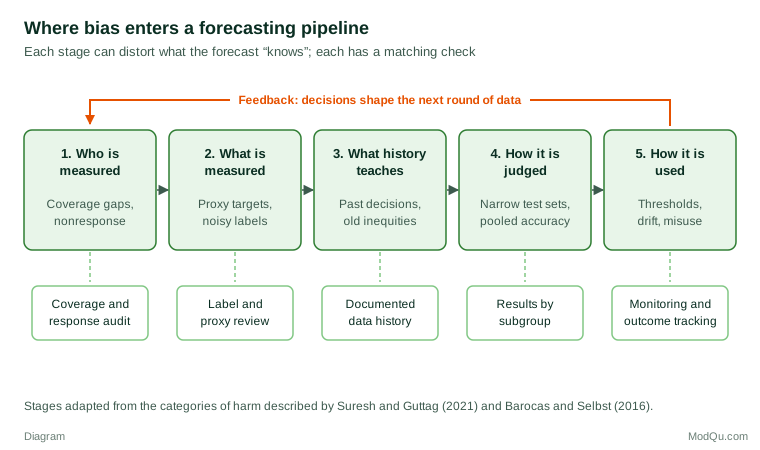
Suresh and Guttag (2021) distinguish several sources of harm across the life cycle of a model, including historical, representation, measurement, aggregation, evaluation and deployment bias. Mehrabi et al. (2021) catalogue a longer list in their survey. For practical purposes, the sources can be grouped into the five stages shown in Figure 1, each with a matching check.
Stage 1: who is measured
Every forecast is built on a sample, even when that sample contains millions of records. Survey methodologists have long organised the ways a sample can misrepresent its population under the framework of total survey error, which includes coverage error, sampling error, nonresponse and measurement error (Groves & Lyberg, 2010). The same framework applies to the data behind an algorithm. Customer databases cover only customers. Web panels and app data over-represent people who are online and willing to share. Bethlehem (2010) shows how undercoverage and self-selection in web surveys produce selection bias that weighting cannot always remove.
Size does not cure this. Meng (2018) demonstrated that when the chance of being included in a dataset is even slightly correlated with the quantity being measured, a very large non-random dataset can carry no more information than a small random sample.
Buolamwini and Gebru (2018) give a vivid example of representation bias. Commercial gender classification systems they audited had error rates of up to 34.7% for darker-skinned women, compared with at most 0.8% for lighter-skinned men. The systems had been trained and benchmarked on image collections in which some groups were scarce, so their accuracy was effectively measured on the people they already served well.
Stage 2: what is measured
Algorithms forecast whatever target they are given. Often the real quantity of interest cannot be observed, so a proxy is used instead. This choice of target variable is one of the most consequential and least scrutinised decisions in a project (Barocas & Selbst, 2016).
Obermeyer et al. (2019) studied a widely used algorithm that identified patients for extra care by predicting their future healthcare costs. Cost was a convenient proxy for need, but less money had historically been spent on Black patients with the same level of illness. As a result, at any given risk score Black patients were considerably sicker than White patients. The authors estimated that correcting the disparity would raise the share of Black patients selected for additional help from 17.7% to 46.5%. The model was accurate about costs; it was biased about need, which was what decision-makers believed it measured.
Business analogues are common: a "satisfaction" model trained on complaint records learns who complains, not who is dissatisfied.
Stage 3: what history teaches
Even with good coverage and a well-chosen target, historical data record the results of earlier decisions. If one group was given fewer loans in the past, the data contain fewer examples of that group repaying loans. If police patrolled some neighbourhoods more heavily, more crime was recorded there.
Lum and Isaac (2016) applied a predictive policing algorithm to recorded drug crimes in Oakland, California. Public health survey estimates suggested that drug use was spread widely across the city, but the algorithm directed patrols mainly to neighbourhoods with more Black and low-income residents, because that was where past enforcement had produced records. Ensign et al. (2018) showed formally how such systems can create runaway feedback loops: patrols are sent where crime was observed, more crime is observed where patrols are sent, and the forecast confirms itself regardless of the true crime rates. This is the feedback arrow in Figure 1.
Observational data describe the system that produced them, not a neutral reality. A forecast trained on them may describe past practice accurately while being a poor guide to different practice.
Stage 4: how the forecast is judged
A model is usually evaluated on a held-out test set and summarised by one number such as accuracy or the area under the ROC curve. If the test set shares the coverage problems of the training data, the evaluation repeats them. If the summary is pooled across groups, large differences in error rates can disappear.
Hand (2006) adds a caution about the evaluation of predictive methods in general. Much of the apparent superiority of sophisticated classifiers over simple ones, he argues, disappears in practice once population drift, sample selection and uncertainty about the costs of errors are taken into account. Dressel and Farid (2018) found that a commercial tool used to predict reoffending was about as accurate as the predictions of people with little or no criminal justice expertise, and no more accurate than a simple model using two variables. A complex model is not automatically better informed, and its complexity can make its errors harder to see.
Stage 5: how the forecast is used
A forecast becomes a decision when someone sets a threshold, chooses whom to act on and decides what action to take. The population the model meets after deployment may differ from the one it was trained on, a problem known as dataset shift. Moreno-Torres et al. (2012) distinguish shift in the predictors, in the prevalence of the outcome and in the relationship between them; each can quietly degrade a model's accuracy for some groups more than others.
Lazer et al. (2014) describe how Google Flu Trends, which forecast influenza from search queries, came to predict more than double the proportion of doctor visits for influenza-like illness reported by the US Centers for Disease Control and Prevention. Changes in search behaviour and in the search engine itself broke the relationship the model relied on. The episode shows that a forecast's knowledge is tied to the conditions under which it was learned.
The fairness trade-off: a worked example
Suppose an analyst wants a forecast to be fair. Three natural requirements suggest themselves:
- Calibration within groups. Among customers given a 70% risk score, about 70% should actually churn, whatever group they belong to.
- Equal false positive rates. Customers who will not churn should be wrongly flagged equally often in each group.
- Equal false negative rates. Customers who will churn should be missed equally often in each group.
Kleinberg et al. (2017) proved that, except in trivial cases, these conditions cannot all hold at once when the groups have different base rates. Chouldechova (2017) reached the same conclusion for recidivism instruments: a score with equal predictive value across groups must have unequal error rates if the groups' underlying rates differ.
Figure 2 shows the result with illustrative numbers. A churn model gives each customer one of three risk scores: 10%, 40% or 70%. The scores are perfectly calibrated in both groups, and the business contacts every customer with a score of 50% or more. In hypothetical Group A, 600 customers score 10%, 300 score 40% and 100 score 70%, giving a churn rate of 25%. In Group B the counts are 300, 300 and 400, giving a churn rate of 43%.
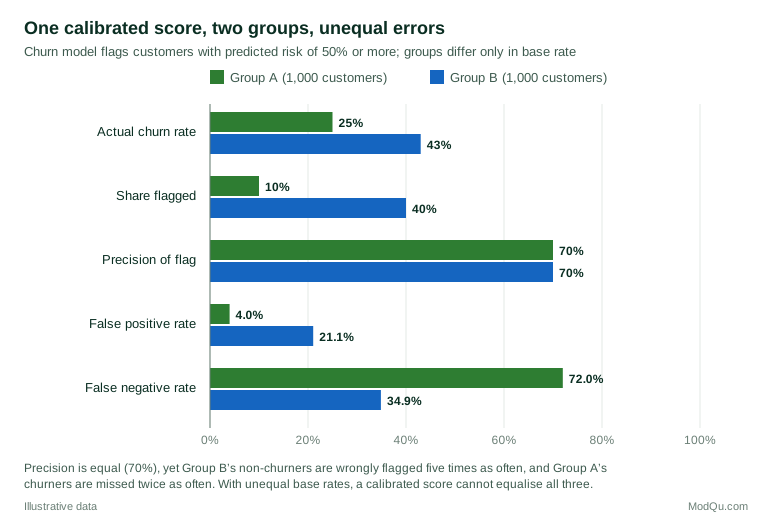
In both groups, 70% of flagged customers really do churn, so the flag is equally reliable. But Group B's loyal customers are wrongly flagged 21.1% of the time against 4.0% in Group A, and Group A's churners are missed 72.0% of the time against 34.9% in Group B. Changing the threshold for one group can equalise the error rates, but only by giving the same score a different meaning depending on group membership.
Corbett-Davies et al. (2017) frame this as a choice between objectives: applying a single threshold to calibrated scores maximises the immediate benefit of the decisions, while imposing equal error rates has a measurable cost in that benefit. Which criterion matters most depends on the decision. If the "flag" is a discount offer, false positives are cheap; if it is a credit refusal or a fraud investigation, they may be serious. Statistics can make the trade-off visible and quantify it, but it cannot settle which harm is worse. That is a judgement for the organisation, ideally made openly and with the people affected in mind.
Why this is an epistemic problem as well as an ethical one
It is tempting to treat fairness as a constraint added after the "real" statistical work is done. The examples above suggest otherwise. In each case the biased forecast was also a poor piece of knowledge: it measured the wrong thing, described the wrong population, mistook past practice for underlying reality or stopped working when conditions changed. Box (1976) reminded statisticians that every model is an approximation and that the skill lies in knowing where it is importantly wrong. Algorithmic bias is often a model being importantly wrong for a particular group.
A score is also a claim made by the people who built and deployed it. The American Statistical Association (2022) asks practitioners to be transparent about methods and limitations and to consider how their work affects the people and communities it concerns. Those duties do not lapse because a computation is automated.
Practical guidance for survey and business data
- Audit coverage before modelling. Compare the training data with the population the forecast will be applied to, using census or reference survey benchmarks where possible. Note which groups are thin or missing.
- Interrogate the target. Ask what the label really measures and how it was produced. Where a proxy is used, test whether its relationship with the true outcome differs across groups.
- Report results by subgroup. Show calibration, false positive and false negative rates for relevant groups, not only pooled accuracy. Model cards provide a structured format for this (Mitchell et al., 2019).
- Document the data. Datasheets record why a dataset was created, how it was collected and what it should not be used for (Gebru et al., 2021). For survey data, include the sampling design, response rates and weighting.
- Prefer simple, inspectable models when stakes are high. If a simple model performs nearly as well, its errors are easier to explain and challenge (Hand, 2006).
- Monitor after deployment. Track outcomes for flagged and unflagged cases, watch for shifts in the population and in the meaning of predictors, and look for feedback loops in which the forecast changes the data it will later learn from.
- Make trade-offs explicit. State which fairness criterion was prioritised and why, and what that choice costs.
Common mistakes
- Removing the protected variable and declaring the model fair. Other variables, such as postcode or purchase history, often act as proxies, so the pattern remains (Barocas & Selbst, 2016).
- Assuming big data are representative. Volume reduces sampling error, not selection bias (Meng, 2018).
- Reporting one accuracy figure. Pooled metrics can conceal large differences between groups.
- Treating fairness as a single number. The main criteria conflict; choosing among them is a decision, not a calculation.
Key takeaways
Algorithmic forecasts are statistical knowledge claims, and they inherit the weaknesses of the data, labels and history behind them. Bias can enter when deciding who is measured, what is measured, what the past teaches, how the model is judged and how it is used. Because common fairness criteria cannot all be met when base rates differ, every deployed forecast embodies a choice about whose errors matter most. Responsible practice makes that choice visible: audit coverage, question proxies, report results by group, document data and models, and keep watching once the forecast is in use.
References
American Statistical Association. (2022). Ethical guidelines for statistical practice. American Statistical Association, Committee on Professional Ethics.
Barocas, S., & Selbst, A. D. (2016). Big data's disparate impact. California Law Review, 104(3), 671–732. https://doi.org/10.15779/Z38BG31
Bethlehem, J. (2010). Selection bias in web surveys. International Statistical Review, 78(2), 161–188. https://doi.org/10.1111/j.1751-5823.2010.00112.x
Box, G. E. P. (1976). Science and statistics. Journal of the American Statistical Association, 71(356), 791–799. https://doi.org/10.1080/01621459.1976.10480949
Buolamwini, J., & Gebru, T. (2018). Gender shades: Intersectional accuracy disparities in commercial gender classification. In Proceedings of the 1st Conference on Fairness, Accountability and Transparency (Proceedings of Machine Learning Research, Vol. 81, pp. 77–91). PMLR.
Chouldechova, A. (2017). Fair prediction with disparate impact: A study of bias in recidivism prediction instruments. Big Data, 5(2), 153–163. https://doi.org/10.1089/big.2016.0047
Corbett-Davies, S., Pierson, E., Feller, A., Goel, S., & Huq, A. (2017). Algorithmic decision making and the cost of fairness. In Proceedings of the 23rd ACM SIGKDD International Conference on Knowledge Discovery and Data Mining (pp. 797–806). ACM. https://doi.org/10.1145/3097983.3098095
Dressel, J., & Farid, H. (2018). The accuracy, fairness, and limits of predicting recidivism. Science Advances, 4(1), Article eaao5580. https://doi.org/10.1126/sciadv.aao5580
Ensign, D., Friedler, S. A., Neville, S., Scheidegger, C., & Venkatasubramanian, S. (2018). Runaway feedback loops in predictive policing. In Proceedings of the 1st Conference on Fairness, Accountability and Transparency (Proceedings of Machine Learning Research, Vol. 81, pp. 160–171). PMLR.
Gebru, T., Morgenstern, J., Vecchione, B., Vaughan, J. W., Wallach, H., Daumé, H., III, & Crawford, K. (2021). Datasheets for datasets. Communications of the ACM, 64(12), 86–92. https://doi.org/10.1145/3458723
Groves, R. M., & Lyberg, L. (2010). Total survey error: Past, present, and future. Public Opinion Quarterly, 74(5), 849–879. https://doi.org/10.1093/poq/nfq065
Hand, D. J. (2006). Classifier technology and the illusion of progress. Statistical Science, 21(1), 1–14. https://doi.org/10.1214/088342306000000060
Kleinberg, J., Mullainathan, S., & Raghavan, M. (2017). Inherent trade-offs in the fair determination of risk scores. In C. H. Papadimitriou (Ed.), 8th Innovations in Theoretical Computer Science Conference (ITCS 2017) (Leibniz International Proceedings in Informatics, Vol. 67, pp. 43:1–43:23). Schloss Dagstuhl–Leibniz-Zentrum für Informatik. https://doi.org/10.4230/LIPIcs.ITCS.2017.43
Lazer, D., Kennedy, R., King, G., & Vespignani, A. (2014). The parable of Google Flu: Traps in big data analysis. Science, 343(6176), 1203–1205. https://doi.org/10.1126/science.1248506
Lum, K., & Isaac, W. (2016). To predict and serve? Significance, 13(5), 14–19. https://doi.org/10.1111/j.1740-9713.2016.00960.x
Mehrabi, N., Morstatter, F., Saxena, N., Lerman, K., & Galstyan, A. (2021). A survey on bias and fairness in machine learning. ACM Computing Surveys, 54(6), Article 115. https://doi.org/10.1145/3457607
Meng, X.-L. (2018). Statistical paradises and paradoxes in big data (I): Law of large populations, big data paradox, and the 2016 US presidential election. The Annals of Applied Statistics, 12(2), 685–726. https://doi.org/10.1214/18-AOAS1161SF
Mitchell, M., Wu, S., Zaldivar, A., Barnes, P., Vasserman, L., Hutchinson, B., Spitzer, E., Raji, I. D., & Gebru, T. (2019). Model cards for model reporting. In Proceedings of the Conference on Fairness, Accountability, and Transparency (pp. 220–229). ACM. https://doi.org/10.1145/3287560.3287596
Moreno-Torres, J. G., Raeder, T., Alaiz-Rodríguez, R., Chawla, N. V., & Herrera, F. (2012). A unifying view on dataset shift in classification. Pattern Recognition, 45(1), 521–530. https://doi.org/10.1016/j.patcog.2011.06.019
Obermeyer, Z., Powers, B., Vogeli, C., & Mullainathan, S. (2019). Dissecting racial bias in an algorithm used to manage the health of populations. Science, 366(6464), 447–453. https://doi.org/10.1126/science.aax2342
Suresh, H., & Guttag, J. (2021). A framework for understanding sources of harm throughout the machine learning life cycle. In Equity and Access in Algorithms, Mechanisms, and Optimization (EAAMO '21) (Article 17). ACM. https://doi.org/10.1145/3465416.3483305