
Statistics · Tests and models
Simple and Multiple Linear Regression
How simple and multiple linear regression describe a numeric outcome, how to read coefficients and R², which assumptions matter most, and how to apply regression soundly to survey and business data.
Linear regression is the workhorse of applied statistics. It tells an analyst how much a numeric outcome, such as monthly spending, time on site or a satisfaction index, changes on average with one or more explanatory variables. Simple regression uses one predictor; multiple regression uses several at once, which allows each effect to be estimated while the others are held constant. Many more advanced methods, including logistic, ordinal and multilevel models, are extensions of the same idea.
Origins
The name comes from Francis Galton, who found that the children of unusually tall parents were, on average, less tall than their parents, and the children of short parents less short. He called this "regression towards mediocrity" (Galton, 1886), a phenomenon now known as regression to the mean. The fitting method is older: Legendre published the method of least squares in 1805, and Gauss developed its probabilistic justification soon afterwards (Stigler, 1986). The combination of the two ideas gave the regression model used today.
The simple linear regression model
Simple linear regression describes the outcome y as a straight-line function of one predictor x plus an error term:
yi = β0 + β1xi + εi
The intercept β0 is the expected outcome when x is zero, and the slope β1 is the expected change in y for a one-unit increase in x. The error εi collects everything else that affects respondent i. Ordinary least squares (OLS) chooses the estimates that make the sum of squared residuals, Σ(yi − ŷi)², as small as possible, where ŷi is the fitted value and the residual yi − ŷi is the vertical distance between a point and the line.
The coefficient of determination, R², is the share of the variance in y accounted for by the model. In simple regression it equals the square of Pearson's correlation between x and y. The residual standard deviation is often more useful for business audiences, because it is in the outcome's own units and shows how far typical observations fall from their predicted values.
Worked example: spend and satisfaction
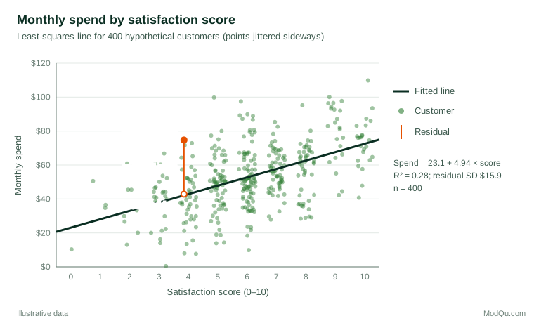
Consider a hypothetical survey of 400 customers of a subscription service, linked to their monthly spend. Regressing spend on a 0–10 satisfaction score gives:
predicted spend = $23.1 + $4.94 × satisfaction
Each extra point of satisfaction is associated with $4.94 more monthly spend on average (95% confidence interval $4.15 to $5.73). The intercept, $23.1, is the predicted spend at a score of zero, a value at the edge of the data that should not be over-interpreted. R² is 0.28, so satisfaction accounts for 28% of the variation in spend, and the residual standard deviation is $15.9 (Figure 1).
Multiple linear regression
Multiple regression extends the model to k predictors:
yi = β0 + β1x1i + β2x2i + … + βkxki + εi
Each coefficient now describes the expected change in y for a one-unit change in that predictor when the other predictors are held constant. This is what makes multiple regression valuable: it separates the contributions of variables that are themselves related.
In the example, longer-standing customers both spend more and tend to be more satisfied (the correlation between tenure and satisfaction is 0.51). Adding tenure in years to the model gives:
predicted spend = $23.8 + $2.77 × satisfaction + $2.62 × tenure
Among customers with the same tenure, one extra satisfaction point is now associated with $2.77 more spend (95% interval $1.95 to $3.59), little more than half the simple estimate. Part of the original association reflected tenure. Each extra year of tenure is associated with $2.62 more spend at a given satisfaction level. R² rises to 0.43 and the residual standard deviation falls to $14.2. A customer with a satisfaction score of 8 and five years' tenure has a predicted spend of about $59.
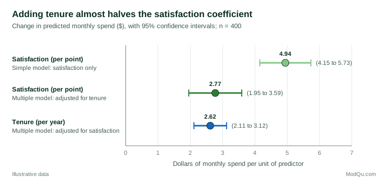
This change is typical rather than unusual. Whenever predictors are correlated, adding or removing one changes the others' coefficients. Omitting an important variable that is related to both a predictor and the outcome biases the predictor's coefficient, which is a form of confounding. Adding variables that are consequences of the outcome, or of the predictor of interest, can introduce bias of its own. Choosing predictors therefore requires subject-matter reasoning, not only statistical fit.
Reading regression output
Statistical software reports, for each coefficient, an estimate, a standard error, a t statistic (the estimate divided by its standard error) and a p-value for the hypothesis that the true coefficient is zero. In the multiple model, the satisfaction coefficient of 2.77 has a standard error of 0.42, giving t ≈ 6.6, far beyond what chance alone would plausibly produce. The 95% confidence interval, roughly the estimate plus or minus two standard errors, is more informative than the p-value because it shows the range of effect sizes consistent with the data.
The output also includes an F test of whether the predictors jointly explain any variation, and an adjusted R², which penalises the ordinary R² for the number of predictors. Adjusted R² is 0.42 in the multiple model, almost identical to the unadjusted value because two predictors are few relative to 400 respondents. With many predictors and a small sample, the gap widens, warning that part of the apparent fit is noise.
Two kinds of interval are easily confused. A confidence interval for the mean spend of all customers with a score of 8 and five years' tenure is narrow, because it reflects only uncertainty in the coefficients. A prediction interval for one new customer with those values is much wider, because it adds the individual variation measured by the residual standard deviation of $14.2: roughly $59 plus or minus $28. Forecasts for individual customers should use the second.
Categorical predictors and interactions
Categorical variables such as region or plan type enter the model as indicator (dummy) variables, one for each category except a reference category; each coefficient is then a difference from that reference group. An interaction term, the product of two predictors, allows the effect of one to depend on the level of the other, for example if satisfaction matters more for new customers than long-standing ones. Curved relationships can be modelled with polynomial terms or splines while keeping the model linear in its coefficients (Harrell, 2015).
Assumptions, in order of importance
Textbooks often list normality first, but Gelman et al. (2020) argue that the assumptions matter in roughly this order:
- Validity. The outcome and predictors measure what the question is about, and the model includes the variables needed to answer it.
- Representativeness. The sample represents the population of interest, or weights and adjustments make it so.
- Linearity and additivity. The expected outcome is a linear function of the predictors as entered. Check with plots of residuals against fitted values and against each predictor.
- Independence of errors. Respondents in the same household, store or interviewer cluster are not independent, and time series usually have correlated errors.
- Equal variance. The spread of residuals is similar across fitted values. Spending data often show a funnel shape, with larger residuals for bigger spenders.
- Normality of errors. This matters for prediction intervals and in small samples, but with a few hundred observations, tests and intervals for coefficients are fairly robust to non-normal errors (Lumley et al., 2002).
When the variance is unequal, heteroscedasticity-consistent standard errors (White, 1980) keep inference valid without changing the coefficients. Long and Ervin (2000) recommend the HC3 version, particularly in samples of fewer than 250. For strongly skewed outcomes such as spend or income, a log transformation, or a more general power transformation chosen by the method of Box and Cox (1964), can make the relationship more linear and the variance more stable, at the cost of coefficients that describe proportional rather than absolute changes.
Diagnostics
Good practice is to plot the data before fitting and the residuals after. Anscombe (1973) showed four data sets with identical regression lines and R² values but entirely different patterns, only one of which suited a straight line. Useful checks include:
- Residual plots for curvature, funnels and clusters.
- Influence measures such as Cook's (1977) distance, which shows how much the fitted coefficients would change if a single observation were removed. Influential points should be checked for errors, not deleted automatically; robust regression methods reduce their impact when they are genuine (Rousseeuw & Leroy, 1987).
- Multicollinearity. When predictors are highly correlated, their individual coefficients become imprecise even if the model predicts well. Variance inflation factors (VIFs) measure this; in the example the VIF is only 1.35. Common thresholds such as 10 should not be applied mechanically, because the precision of a coefficient also depends on sample size and residual variance (O'Brien, 2007).
Practical guidance for survey and business data
- Sample size. For estimating regression coefficients, a simulation study by Austin and Steyerberg (2015) found that as few as two observations per predictor gave little bias in linear regression. Precise estimates, subgroup analyses and good out-of-sample prediction require far more, and models with many predictors relative to the sample are prone to overfitting (Harrell, 2015).
- Survey weights and design. For estimates intended to describe a population, fit the model with the survey weights and design-based standard errors (Lumley, 2010). Solon et al. (2015) explain when weighting changes regression results and recommend comparing weighted and unweighted estimates as a diagnostic: a large difference suggests the model is misspecified or effects vary across groups.
- Rating scales as predictors or outcomes. Treating a 0–10 rating as numeric is common and usually reasonable. For outcomes with few ordered categories, ordinal regression is often better.
- Keep continuous predictors continuous. Splitting age or income into two groups loses information and can produce misleading results (MacCallum et al., 2002).
- Compare predictors on a sensible scale. Raw coefficients depend on units. Gelman (2008) suggests dividing continuous predictors by two standard deviations so that their coefficients are comparable with those of binary predictors.
- Look beyond the average. Quantile regression estimates how predictors relate to the lower or upper parts of the outcome distribution, for example to heavy spenders specifically (Koenker & Hallock, 2001).
- Be clear about the goal. Breiman (2001) distinguished modelling to understand how data are generated from modelling to predict accurately. A model built for prediction can include any useful predictors and should be judged on new data; a model built to explain needs carefully chosen variables and cautious interpretation.
Common mistakes
- Reading coefficients as causal effects. In the example, the data cannot show that raising satisfaction would increase spending; regression on observational survey data shows adjusted associations.
- Extrapolating beyond the range of the data, such as predicting spend for a satisfaction score of 15 or for a market not in the sample.
- Judging a model by R² alone. A low R² can accompany precise, useful coefficients, and a high R² can come from trends or overfitting.
- Comparing raw coefficients for predictors measured in different units.
- Ignoring clustering and weights in survey samples, which usually understates uncertainty.
- Selecting predictors by repeated significance testing, which produces optimistic results that do not replicate.
Key takeaways
Linear regression summarises how a numeric outcome changes with one or more predictors. Simple regression gives the overall association; multiple regression estimates each association with the other predictors held constant, which can change the picture considerably, as the satisfaction coefficient in the example shows. Validity, representativeness and linearity matter more than normality. Plot the data and residuals, use robust or design-based standard errors where needed, report effects in meaningful units with confidence intervals, and remember the advice of Box (1976) that all models are wrong: a useful regression is one whose simplifications are understood and appropriate for the decision at hand.
References
Anscombe, F. J. (1973). Graphs in statistical analysis. The American Statistician, 27(1), 17–21. https://doi.org/10.1080/00031305.1973.10478966
Austin, P. C., & Steyerberg, E. W. (2015). The number of subjects per variable required in linear regression analyses. Journal of Clinical Epidemiology, 68(6), 627–636. https://doi.org/10.1016/j.jclinepi.2014.12.014
Box, G. E. P. (1976). Science and statistics. Journal of the American Statistical Association, 71(356), 791–799. https://doi.org/10.1080/01621459.1976.10480949
Box, G. E. P., & Cox, D. R. (1964). An analysis of transformations. Journal of the Royal Statistical Society Series B: Statistical Methodology, 26(2), 211–243. https://doi.org/10.1111/j.2517-6161.1964.tb00553.x
Breiman, L. (2001). Statistical modeling: The two cultures (with comments and a rejoinder by the author). Statistical Science, 16(3), 199–231. https://doi.org/10.1214/ss/1009213726
Cook, R. D. (1977). Detection of influential observation in linear regression. Technometrics, 19(1), 15–18. https://doi.org/10.1080/00401706.1977.10489493
Galton, F. (1886). Regression towards mediocrity in hereditary stature. The Journal of the Anthropological Institute of Great Britain and Ireland, 15, 246–263. https://doi.org/10.2307/2841583
Gelman, A. (2008). Scaling regression inputs by dividing by two standard deviations. Statistics in Medicine, 27(15), 2865–2873. https://doi.org/10.1002/sim.3107
Gelman, A., Hill, J., & Vehtari, A. (2020). Regression and other stories. Cambridge University Press. https://doi.org/10.1017/9781139161879
Harrell, F. E., Jr. (2015). Regression modeling strategies: With applications to linear models, logistic and ordinal regression, and survival analysis (2nd ed.). Springer. https://doi.org/10.1007/978-3-319-19425-7
Koenker, R., & Hallock, K. F. (2001). Quantile regression. Journal of Economic Perspectives, 15(4), 143–156. https://doi.org/10.1257/jep.15.4.143
Long, J. S., & Ervin, L. H. (2000). Using heteroscedasticity consistent standard errors in the linear regression model. The American Statistician, 54(3), 217–224. https://doi.org/10.1080/00031305.2000.10474549
Lumley, T. (2010). Complex surveys: A guide to analysis using R. Wiley. https://doi.org/10.1002/9780470580066
Lumley, T., Diehr, P., Emerson, S., & Chen, L. (2002). The importance of the normality assumption in large public health data sets. Annual Review of Public Health, 23(1), 151–169. https://doi.org/10.1146/annurev.publhealth.23.100901.140546
MacCallum, R. C., Zhang, S., Preacher, K. J., & Rucker, D. D. (2002). On the practice of dichotomization of quantitative variables. Psychological Methods, 7(1), 19–40. https://doi.org/10.1037/1082-989X.7.1.19
O'Brien, R. M. (2007). A caution regarding rules of thumb for variance inflation factors. Quality & Quantity, 41(5), 673–690. https://doi.org/10.1007/s11135-006-9018-6
Rousseeuw, P. J., & Leroy, A. M. (1987). Robust regression and outlier detection. Wiley. https://doi.org/10.1002/0471725382
Solon, G., Haider, S. J., & Wooldridge, J. M. (2015). What are we weighting for? Journal of Human Resources, 50(2), 301–316. https://doi.org/10.3368/jhr.50.2.301
Stigler, S. M. (1986). The history of statistics: The measurement of uncertainty before 1900. Belknap Press of Harvard University Press.
White, H. (1980). A heteroskedasticity-consistent covariance matrix estimator and a direct test for heteroskedasticity. Econometrica, 48(4), 817–838. https://doi.org/10.2307/1912934