
Statistics · Descriptive statistics
Robust Statistics for Messy and Outlier-Prone Data
Why one bad value can wreck a mean, and how medians, trimmed means, robust spreads and robust outlier rules give stable answers from survey and business data that are less than perfectly clean.
Real data are rarely tidy. A respondent types 950 instead of 95, a few very large customers dominate a spending question, a panellist speeds through a grid, or a sensor sends a burst of nonsense. Classical summaries such as the mean and standard deviation were designed for well-behaved, roughly normal data, and they can be badly misled by even a single unusual value. Robust statistics is the branch of statistics that builds summaries and models which still give sensible answers when a minority of the data are wrong or unusual (Hampel et al., 2005; Rousseeuw & Hubert, 2011). This article explains the main ideas, works through a small example, and gives practical guidance for survey and business data.
Why classical summaries break
The sample mean gives every observation an equal say. That is a virtue when every observation is trustworthy, but it also means that one extreme value can drag the mean as far as it likes. The standard deviation is even more sensitive, because it squares each deviation from the mean. Tukey (1977) built much of his exploratory approach around this problem, favouring medians, quartiles and resistant summaries that are not upset by a few wild points.
Two ideas make "sensitivity" precise. The influence function describes how much an estimate changes when a small amount of contamination is added at a given value (Hampel, 1974). For the mean, the influence of a point grows without limit as the point moves further away; for the median, it is bounded. The breakdown point is the smallest share of the data that, if replaced by arbitrary values, can push the estimate to any value at all (Hampel, 1971). The mean and standard deviation have a breakdown point of zero: one bad value is enough. The median has the highest possible breakdown point, 50%, because more than half the data must be corrupted before it can be moved arbitrarily far.
In their standard reference work, Hampel et al. (2005) set out the theory that ties these ideas together. A good robust method balances two goals: a high breakdown point and bounded influence, so that bad data cannot take over, and high efficiency, so that little precision is lost when the data are in fact clean.
Robust measures of location
Several estimators of the "typical" value are in routine use:
- Median. The middle value. It has a 50% breakdown point and is easy to explain, but for clean normal data it is less precise than the mean, with an efficiency of about 64%.
- Trimmed mean. Sort the data, remove a fixed share from each end, and average the rest. A 20% trimmed mean removes the lowest and highest 20%. Wilcox and Keselman (2003) argue that 20% trimming is a good general default, combining strong protection against outliers with good efficiency.
- Winsorised mean. Instead of removing the extreme values, replace them with the most extreme values that remain. This keeps the sample size and is common in business surveys.
- Hodges–Lehmann estimator. The median of all pairwise averages of the observations, derived from rank tests (Hodges & Lehmann, 1963). It is robust and nearly as efficient as the mean for normal data.
- M-estimators. Huber (1964) proposed estimators that treat small deviations like the mean but give less weight to large ones. With the common tuning constant of 1.345 (in units of a robust standard deviation), the Huber estimator keeps about 95% of the mean's efficiency for normal data while limiting the influence of outliers (Wilcox, 2022).
Robust measures of spread
Spread needs the same protection. The interquartile range (IQR), the distance between the first and third quartiles, has a breakdown point of 25%. The median absolute deviation (MAD) is the median of the absolute distances from the median, and it has a breakdown point of 50%. Multiplying the MAD by 1.4826 gives the "normalised" MAD, which estimates the standard deviation when the data are normal. Rousseeuw and Croux (1993) proposed two alternatives, called Sn and Qn, that keep the 50% breakdown point but are more efficient than the MAD and do not assume a symmetric distribution.
MADN = 1.4826 × median( | xi − median(x) | )
A worked example
Suppose a hypothetical survey asks 12 customers for their monthly spend in a category. The correct answers are $42, 48, 51, 55, 58, 60, 63, 67, 70, 74, 81 and 95. During data entry, the $95 is mistyped as $950. The table compares common summaries for the clean and the contaminated data.
| Summary (illustrative data) | Correct data | With $950 typo |
|---|---|---|
| Mean | $63.7 | $134.9 |
| Median | $61.5 | $61.5 |
| 20% trimmed mean | $62.2 | $62.2 |
| Winsorised mean (one value each end) | $63.0 | $63.0 |
| Huber M-estimate (k = 1.345) | $62.7 | $62.7 |
| Standard deviation | $14.9 | $256.9 |
| Normalised MAD | $14.1 | $14.1 |
| Interquartile range | $17.0 | $17.0 |
One error more than doubles the mean and multiplies the standard deviation by about 17. Every robust summary is unchanged, because the typo simply replaces one extreme value with another extreme value, and none of them depend on how extreme it is. The mean of $134.9 is also a poor description of anyone: it is higher than every genuine response in the sample.
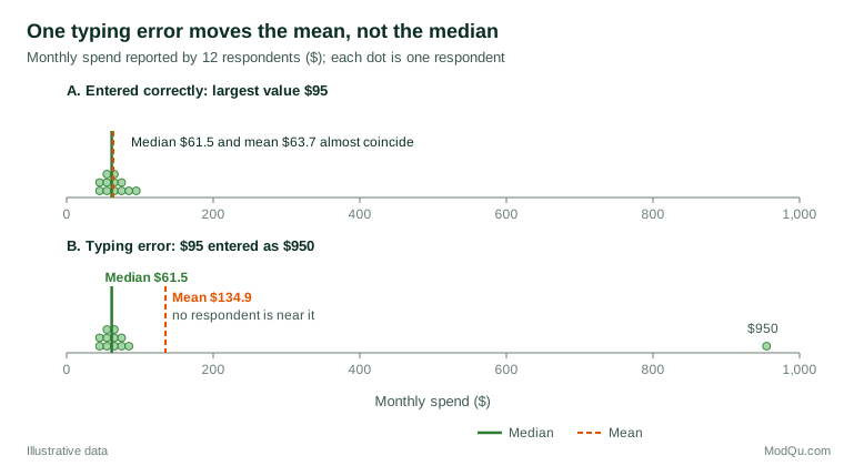
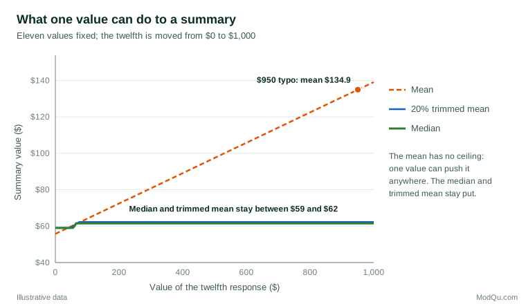
Figure 2 generalises the example. It holds eleven responses fixed and moves the twelfth from $0 to $1,000. The mean follows it in a straight line with no ceiling. The median and the 20% trimmed mean move only while the twelfth value is among the central observations and then stay flat, whatever the value. This is the bounded influence that Hampel (1974) formalised.
Detecting outliers robustly
A popular rule flags any value more than three standard deviations from the mean. The rule has a basic flaw: the outliers inflate the very mean and standard deviation used to judge them, so they can hide themselves. This is called masking. In the example, the $950 has a z-score of only 3.17. In fact, in a sample of 12 no value can ever have a z-score above (n − 1) ÷ √n ≈ 3.18, however extreme it is (Shiffler, 1988). In small samples, a "three standard deviations" rule is therefore close to useless.
Robust rules avoid masking by measuring distance with robust summaries:
- Median and MAD rule. Flag values whose distance from the median exceeds 2.5 or 3 times the normalised MAD. Leys et al. (2013) recommend this rule over the mean-and-standard-deviation rule, with 2.5 as a reasonable default. For the $950 the robust distance is about 63, an unmistakable flag; the genuine $95 scores about 2.4 and is not flagged.
- Boxplot fences. Tukey (1977) flags values more than 1.5 IQRs beyond the quartiles. In the example the upper fence is about $96.5. Quartile conventions differ between software packages, so fences can shift slightly.
- Skewed data. Spending, revenue and time-on-task are usually right-skewed, and the standard fences then flag many genuine large values. The adjusted boxplot of Hubert and Vandervieren (2008) widens the fences on the long side using a robust measure of skewness.
- Several variables at once. A respondent can be unremarkable on each question but unusual in combination. The minimum covariance determinant estimator finds the most tightly clustered subset of the data and measures every case's distance from it; a fast algorithm makes it practical for large files (Rousseeuw & Van Driessen, 1999). Rousseeuw and Hubert (2011) give an accessible overview of these methods.
Beyond descriptive summaries
The same logic extends to models. Ordinary least squares regression has a breakdown point of zero, so a single badly placed point can tilt a fitted line. High-breakdown methods such as least median of squares (Rousseeuw, 1984) and the wider family described by Rousseeuw and Leroy (1987) fit the bulk of the data and then reveal the points that do not follow it. For comparing two groups, Yuen's (1974) test compares trimmed means and allows unequal variances; Wilcox (2022) covers robust versions of most standard tests. Erceg-Hurn and Mirosevich (2008) explain why these methods often have more power than classical tests when data are skewed or heavy-tailed, and how to run them in common software.
Practical guidance for survey and business data
- Look first. Plot every key numeric variable before summarising it. A dot plot or boxplot shows problems that a table of means hides.
- Separate errors from genuine extremes. Aguinis et al. (2013) distinguish error outliers, such as typos and impossible values, from interesting outliers that are genuine and may be the most important cases in the data. Correct or remove errors with a documented rule; never delete genuine large customers just because they are inconvenient.
- Report a robust summary next to the mean. For skewed quantities such as spend, income or time, report the median or a trimmed mean alongside the mean. A large gap between them is itself a finding.
- Remember totals. When the goal is a population total, such as total market spend, the mean matters because totals are means multiplied by population size. Survey statisticians therefore use outlier-robust estimators that limit, rather than remove, the influence of extreme units (Chambers, 1986).
- Account for weights. In a weighted survey, a moderately large value carried by a very large weight can be as influential as an extreme value. Check the product of value and weight, not the value alone.
- Set rules before seeing results. Decide trimming levels and outlier rules in advance and apply them the same way across waves, so that trends are not created by changing choices.
Common mistakes
- Deleting outliers and then testing as if nothing happened. Removing points changes the standard errors. Use methods designed for trimmed data, such as Yuen's test, rather than an ordinary t-test on what is left (Wilcox, 2022).
- Relying on the three-standard-deviation rule. Because of masking, it misses outliers in exactly the situations where they matter most.
- Treating "robust" as "correct". A robust estimate answers a slightly different question from the mean. A median spend is not a substitute for average spend when the business needs a total.
- Hiding the decision. Readers should be told how many values were flagged, what rule was used, and how much the results change.
Key takeaways
Classical summaries trust every value equally, so a single error or extreme case can distort them without limit. Robust statistics gives bounded influence and a high breakdown point at a modest cost in efficiency. In practice, plot the data, report a median or trimmed mean alongside the mean, flag outliers with the median and MAD or adjusted boxplot rules rather than the mean and standard deviation, and document every correction. These habits make results from messy survey and business data far more stable and far easier to defend.
References
Aguinis, H., Gottfredson, R. K., & Joo, H. (2013). Best-practice recommendations for defining, identifying, and handling outliers. Organizational Research Methods, 16(2), 270–301. https://doi.org/10.1177/1094428112470848
Chambers, R. L. (1986). Outlier robust finite population estimation. Journal of the American Statistical Association, 81(396), 1063–1069. https://doi.org/10.1080/01621459.1986.10478374
Erceg-Hurn, D. M., & Mirosevich, V. M. (2008). Modern robust statistical methods: An easy way to maximize the accuracy and power of your research. American Psychologist, 63(7), 591–601. https://doi.org/10.1037/0003-066X.63.7.591
Hampel, F. R. (1971). A general qualitative definition of robustness. The Annals of Mathematical Statistics, 42(6), 1887–1896. https://doi.org/10.1214/aoms/1177693054
Hampel, F. R. (1974). The influence curve and its role in robust estimation. Journal of the American Statistical Association, 69(346), 383–393. https://doi.org/10.1080/01621459.1974.10482962
Hampel, F. R., Ronchetti, E. M., Rousseeuw, P. J., & Stahel, W. A. (2005). Robust statistics: The approach based on influence functions. Wiley. https://doi.org/10.1002/9781118186435
Hodges, J. L., Jr., & Lehmann, E. L. (1963). Estimates of location based on rank tests. The Annals of Mathematical Statistics, 34(2), 598–611. https://doi.org/10.1214/aoms/1177704172
Huber, P. J. (1964). Robust estimation of a location parameter. The Annals of Mathematical Statistics, 35(1), 73–101. https://doi.org/10.1214/aoms/1177703732
Hubert, M., & Vandervieren, E. (2008). An adjusted boxplot for skewed distributions. Computational Statistics & Data Analysis, 52(12), 5186–5201. https://doi.org/10.1016/j.csda.2007.11.008
Leys, C., Ley, C., Klein, O., Bernard, P., & Licata, L. (2013). Detecting outliers: Do not use standard deviation around the mean, use absolute deviation around the median. Journal of Experimental Social Psychology, 49(4), 764–766. https://doi.org/10.1016/j.jesp.2013.03.013
Rousseeuw, P. J. (1984). Least median of squares regression. Journal of the American Statistical Association, 79(388), 871–880. https://doi.org/10.1080/01621459.1984.10477105
Rousseeuw, P. J., & Croux, C. (1993). Alternatives to the median absolute deviation. Journal of the American Statistical Association, 88(424), 1273–1283. https://doi.org/10.1080/01621459.1993.10476408
Rousseeuw, P. J., & Hubert, M. (2011). Robust statistics for outlier detection. WIREs Data Mining and Knowledge Discovery, 1(1), 73–79. https://doi.org/10.1002/widm.2
Rousseeuw, P. J., & Leroy, A. M. (1987). Robust regression and outlier detection. Wiley. https://doi.org/10.1002/0471725382
Rousseeuw, P. J., & Van Driessen, K. (1999). A fast algorithm for the minimum covariance determinant estimator. Technometrics, 41(3), 212–223. https://doi.org/10.1080/00401706.1999.10485670
Shiffler, R. E. (1988). Maximum Z scores and outliers. The American Statistician, 42(1), 79–80. https://doi.org/10.1080/00031305.1988.10475530
Tukey, J. W. (1977). Exploratory data analysis. Addison-Wesley.
Wilcox, R. R. (2022). Introduction to robust estimation and hypothesis testing (5th ed.). Elsevier. https://doi.org/10.1016/C2019-0-01225-3
Wilcox, R. R., & Keselman, H. J. (2003). Modern robust data analysis methods: Measures of central tendency. Psychological Methods, 8(3), 254–274. https://doi.org/10.1037/1082-989X.8.3.254
Yuen, K. K. (1974). The two-sample trimmed t for unequal population variances. Biometrika, 61(1), 165–170. https://doi.org/10.1093/biomet/61.1.165