
Statistics · Causal inference
Regression Discontinuity Designs
How regression discontinuity designs use cut-off rules, such as spend thresholds and eligibility scores, to estimate causal effects, and how to check that the comparison at the threshold is credible.
Many decisions in business and public policy follow a cut-off rule. Customers who spend $1,000 in a year receive Gold status. Applicants who score 70 or more are approved. Schools must split classes once enrolment passes a fixed number. A regression discontinuity design exploits such rules. People just above and just below the threshold are very similar, yet only those above it receive the treatment. Comparing outcomes on either side of the line therefore comes close to a randomised comparison, for the people near the cut-off.
The design was introduced by Thistlethwaite and Campbell (1960), who used it to study the effect of receiving a certificate of merit in a national scholarship competition on students' later aspirations. It was later formalised in econometrics (Hahn et al., 2001) and is now regarded as one of the most credible designs for causal inference with observational data (Lee & Lemieux, 2010).
How the design works
Three ingredients define the design:
- a running variable (also called the score or forcing variable), such as prior-year spend;
- a threshold c on that variable;
- a treatment that changes at the threshold.
In a sharp design, everyone at or above the threshold is treated and nobody below it is. The effect is the size of the jump in the expected outcome at the threshold:
τ = limx↓c E[Y | X = x] − limx↑c E[Y | X = x]
The key assumption is continuity: without the treatment, the average outcome would change smoothly as the running variable crosses the threshold. Any sudden jump can then be attributed to the treatment (Hahn et al., 2001).
In a fuzzy design, crossing the threshold changes the probability of treatment but not from 0 to 1, for example because staff can grant Gold status by hand. The jump in the outcome is then divided by the jump in the probability of treatment, an approach equivalent to using the threshold as an instrumental variable. Angrist and Lavy (1999) used a fuzzy design based on a rule capping class size at 40 pupils to estimate the effect of class size on test scores.
A worked example
Suppose a hypothetical retailer gives Gold status, with free delivery and priority service, to customers who spend at least $1,000 in a year. Management wants to know whether Gold status increases retention. Comparing all Gold customers with all others would mislead, because big spenders are more loyal anyway. The regression discontinuity design compares customers who spent, say, $980 with those who spent $1,020.
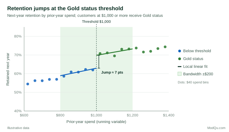
Figure 1 plots the share of customers retained in the following year against prior-year spend, in $40 bins. Retention rises gradually with spend on both sides, but at $1,000 it jumps. Local linear regressions fitted within $200 of the threshold estimate retention of about 63% just below and 70% just above, an effect of about 7 percentage points for customers near the threshold.
For the business, this is a useful but bounded answer. It suggests that Gold status keeps more marginal customers, which helps judge whether the cost of the perks is repaid at the threshold. It does not say whether lowering the threshold to $500 would have the same effect, because customers spending $500 may respond quite differently. A plot like Figure 1 should always accompany the estimate, so that readers can see the jump for themselves.
Estimation choices
Modern practice estimates the jump with local linear regression on each side of the threshold, giving more weight to observations closer to it (Imbens & Lemieux, 2008). Two choices matter most.
- Bandwidth. A narrow window reduces bias, because people are more similar near the threshold, but uses fewer observations and so increases variance. Imbens and Kalyanaraman (2012) derived a data-driven bandwidth that balances the two, and Calonico et al. (2014) showed that conventional confidence intervals at such bandwidths are too narrow and proposed robust bias-corrected intervals, now standard in software.
- Functional form. Fitting high-order polynomials across the whole range of the running variable is a common mistake. Gelman and Imbens (2019) show that such polynomials give noisy estimates, put large weight on points far from the threshold and produce confidence intervals that are too narrow.
Report the estimate across a range of bandwidths so readers can see whether the conclusion depends on one choice.
Checking the design
The continuity assumption cannot be tested directly, but its main threats can be examined.
- Manipulation. If customers know about the threshold, those just short may buy extra items to qualify, and they may differ from those who do not. McCrary (2008) proposed testing whether the density of the running variable jumps at the threshold; a pile-up just above it is a warning sign.
- Covariate balance. Characteristics fixed before the treatment, such as tenure or region, should not jump at the threshold. Lee (2008) used this logic in close elections, where candidates who barely won and barely lost were similar in their earlier characteristics.
- Placebo thresholds. Estimating "effects" at points where nothing changes, such as $800 or $1,200, should give results close to zero.
Practical guidance and limitations
- The estimate is local. It describes customers near $1,000, not those spending $300 or $5,000. Extrapolating it to the whole customer base requires further assumptions.
- Sample size near the threshold matters. Regression discontinuity needs far more data than a randomised experiment of similar precision, because only observations near the cut-off are informative (Lee & Lemieux, 2010).
- Combine with survey data carefully. Linking survey responses on satisfaction or intention to administrative scores works well, but nonresponse that differs on either side of the threshold can mimic a discontinuity.
- Other changes at the same threshold break the design. If $1,000 also triggers a different marketing programme, the jump combines both effects.
Angrist and Pischke (2009) give an accessible introduction to sharp and fuzzy designs alongside related methods.
Key takeaways
Regression discontinuity designs turn arbitrary cut-off rules into credible comparisons. They estimate the treatment effect as the jump in outcomes at the threshold, using local linear regression with a well-chosen bandwidth and robust confidence intervals. Their credibility rests on continuity, which should be supported by density tests, covariate balance and placebo thresholds. The result is precise about a narrow group: people near the cut-off.
References
Angrist, J. D., & Lavy, V. (1999). Using Maimonides' rule to estimate the effect of class size on scholastic achievement. The Quarterly Journal of Economics, 114(2), 533–575. https://doi.org/10.1162/003355399556061
Angrist, J. D., & Pischke, J.-S. (2009). Mostly harmless econometrics: An empiricist's companion. Princeton University Press. https://doi.org/10.1515/9781400829828
Calonico, S., Cattaneo, M. D., & Titiunik, R. (2014). Robust nonparametric confidence intervals for regression-discontinuity designs. Econometrica, 82(6), 2295–2326. https://doi.org/10.3982/ECTA11757
Gelman, A., & Imbens, G. (2019). Why high-order polynomials should not be used in regression discontinuity designs. Journal of Business & Economic Statistics, 37(3), 447–456. https://doi.org/10.1080/07350015.2017.1366909
Hahn, J., Todd, P., & Van der Klaauw, W. (2001). Identification and estimation of treatment effects with a regression-discontinuity design. Econometrica, 69(1), 201–209. https://doi.org/10.1111/1468-0262.00183
Imbens, G., & Kalyanaraman, K. (2012). Optimal bandwidth choice for the regression discontinuity estimator. The Review of Economic Studies, 79(3), 933–959. https://doi.org/10.1093/restud/rdr043
Imbens, G. W., & Lemieux, T. (2008). Regression discontinuity designs: A guide to practice. Journal of Econometrics, 142(2), 615–635. https://doi.org/10.1016/j.jeconom.2007.05.001
Lee, D. S. (2008). Randomized experiments from non-random selection in U.S. House elections. Journal of Econometrics, 142(2), 675–697. https://doi.org/10.1016/j.jeconom.2007.05.004
Lee, D. S., & Lemieux, T. (2010). Regression discontinuity designs in economics. Journal of Economic Literature, 48(2), 281–355. https://doi.org/10.1257/jel.48.2.281
McCrary, J. (2008). Manipulation of the running variable in the regression discontinuity design: A density test. Journal of Econometrics, 142(2), 698–714. https://doi.org/10.1016/j.jeconom.2007.05.005
Thistlethwaite, D. L., & Campbell, D. T. (1960). Regression-discontinuity analysis: An alternative to the ex post facto experiment. Journal of Educational Psychology, 51(6), 309–317. https://doi.org/10.1037/h0044319