
Statistics · Tests and models
Non-Parametric Tests: Mann-Whitney, Wilcoxon and Kruskal-Wallis
How rank-based tests compare groups when data are skewed, ordinal or full of outliers, what the Mann-Whitney, Wilcoxon and Kruskal-Wallis tests actually test, and how to report them well.
Business and survey data rarely look like the tidy bell curves of textbook examples. Customer spend is dominated by a few heavy buyers, time on site has a long right tail, and satisfaction is recorded on five-point scales with heavy ties. The t-test and analysis of variance compare means and rely on shape assumptions that are often doubtful in small samples. Non-parametric tests offer an alternative: the three most widely used work with ranks instead of raw values. This article explains how the Mann-Whitney, Wilcoxon signed-rank and Kruskal-Wallis tests work, what they really test, and how to report them. Hollander et al. (2014) give a full textbook treatment.
What "non-parametric" means
A parametric test assumes the data come from a particular family of distributions, such as the normal, described by a few parameters such as a mean and standard deviation. A non-parametric or distribution-free test makes no such assumption about the shape of the population. Its p-value is valid when the null hypothesis is true, whatever the shape of the distributions, provided the observations are independent and the groups have identical distributions under the null.
Distribution-free is not the same as assumption-free. Rank tests still require independent observations or correctly paired data, and their interpretation depends on how the groups differ.
How ranks work
All three tests begin the same way. The observations are pooled and sorted from smallest to largest. The smallest receives rank 1, the next rank 2, and so on. Tied values receive the average of the ranks they would otherwise occupy, so two respondents tied for third and fourth place each get rank 3.5. The test then asks whether high and low ranks are spread evenly across the groups, or whether one group tends to collect the high ranks.
Ranking has a powerful side effect: an extreme value can only take the largest rank, however far it lies from the rest. A top customer who spends $2,000 instead of $200 does not change the analysis. This makes rank tests resistant to outliers and heavy tails.
The Mann-Whitney U test (Wilcoxon rank-sum test)
Purpose and history
The Mann-Whitney test compares two independent groups. Wilcoxon (1945) proposed the rank-sum version for equal group sizes, and Mann and Whitney (1947) independently developed the U statistic and its distribution for unequal groups. The two are equivalent, so software labels the same test as "Wilcoxon rank-sum" or "Mann-Whitney U".
The statistic
After ranking the pooled data, add up the ranks in group 1 to give R1. Then:
U1 = R1 − n1(n1 + 1) ÷ 2
U1 counts how many of the n1 × n2 possible pairs, one observation from each group, have the group 1 value higher, with ties counting a half. The two U values always add up to n1 × n2. If the groups do not differ, U should be close to half that product. Small samples use the exact distribution of U; larger ones use a normal approximation with a correction for ties.
Worked example
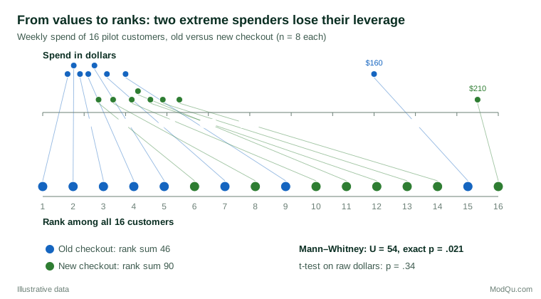
A hypothetical pilot tests a new mobile checkout. Eight customers use the old checkout and eight the new, and the outcome is weekly spend (Figure 1). Each group contains one very heavy spender. The new-checkout group has a rank sum of 90, so U = 90 − 36 = 54 out of a possible 64. The exact two-sided p-value is .021.
A t-test on the raw dollars gives p = .34: the two large values inflate both standard deviations to $50 to $60, hiding the mean difference of about $27. The rank test sees that in 54 of the 64 possible pairings, the new-checkout customer spent more.
What the test actually tests
The Mann-Whitney test is often described as a "test of medians". That description is wrong in general. Its null hypothesis is that the two distributions are identical, and it is sensitive to whether a randomly chosen value from one group tends to exceed a randomly chosen value from the other. Formally, it estimates the probability P(X > Y) + ½P(X = Y) and tests whether it equals one half (Fay & Proschan, 2010).
The test can be read as a comparison of medians only under an extra assumption: that the two distributions have the same shape and differ only by a shift. When shapes or spreads differ, two groups with the same median can produce a significant result, and groups with different medians may not (Divine et al., 2018). Simulation studies by Fagerland and Sandvik (2009) found that, when the aim is to compare means or medians and the groups differ in variance or skewness, the test's error rate can depart considerably from the nominal level.
When spreads differ between groups, the Brunner-Munzel test is a useful alternative. It tests the same probability P(X > Y) without assuming equal distributions under the null (Brunner & Munzel, 2000). In the checkout example it gives p = .015, in line with the Mann-Whitney result.
The Wilcoxon signed-rank test
Purpose
The signed-rank test, also introduced by Wilcoxon (1945), is the non-parametric partner of the paired t-test. Use it when the same respondents are measured twice, such as ratings of two package designs by the same panel, or spending before and after a loyalty programme.
Procedure
- Calculate each respondent's difference between the two conditions.
- Set aside zero differences, or handle them by Pratt's method (Pratt, 1959), which ranks them and then drops their ranks.
- Rank the absolute values of the remaining differences.
- Add the ranks of the positive differences and of the negative differences separately.
If there is no systematic change, the two sums should be similar. A large imbalance suggests that one condition tends to score higher.
The signed-rank test assumes that the differences are symmetric around their centre. Without that assumption it is not simply a test of the median difference. If symmetry is clearly implausible, the sign test, which uses only the direction of each difference, makes fewer assumptions at the cost of power.
With rating scales many differences are zero, and the choice between discarding them and Pratt's method can change the conclusion, so state which was used.
An estimate, not just a p-value
A useful companion to both Wilcoxon tests is the Hodges-Lehmann estimator (Hodges & Lehmann, 1963). For two independent groups it is the median of all pairwise differences between the groups; in the checkout example it is $24.50. For paired data it is the median of all averages of pairs of differences. Unlike a raw difference in medians, it comes with a confidence interval derived from the same rank test.
The Kruskal-Wallis test
Purpose
The Kruskal-Wallis test extends the Mann-Whitney test to three or more independent groups. It is the rank-based counterpart of one-way analysis of variance (Kruskal & Wallis, 1952). The data are pooled and ranked, and the test asks whether the mean ranks differ more between groups than chance would allow:
H = [12 ÷ (N(N + 1))] × Σ (Ri² ÷ ni) − 3(N + 1)
Here N is the total sample size, and Ri and ni are the rank sum and size of group i. With ties, H is divided by a correction factor. For moderate samples H is compared with a chi-square distribution with k − 1 degrees of freedom, where k is the number of groups.
Worked example
A hypothetical retail survey asks 100 customers in each of three regions to rate their satisfaction from 1 to 5 (Figure 2). With only five possible answers, nearly every value is tied.
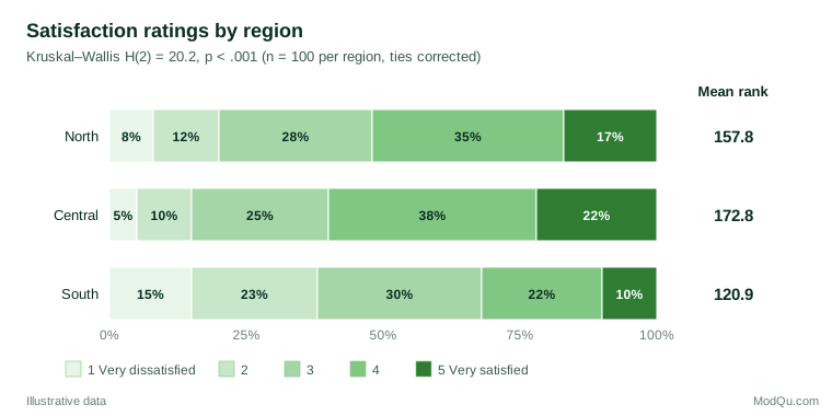
The tie-corrected statistic is H(2) = 20.2, p < .001. The mean ranks are 157.8 for the North, 172.8 for Central and 120.9 for the South. Note that the North and Central regions share the same median rating of 4, yet their mean ranks differ, because Central has more 5s and fewer low ratings. This again shows that rank tests compare whole distributions, not medians.
Following up a significant result
Like the F test, a significant H says only that at least one group differs. Dunn's (1964) procedure compares pairs of groups using the mean ranks from the overall ranking, with a correction for multiple comparisons. Applying it with a Holm adjustment to the example shows that the South differs from Central (adjusted p < .001) and from the North (adjusted p = .004), while the North and Central do not differ significantly (adjusted p = .21). Separate pairwise Mann-Whitney tests re-rank the data each time and are not consistent with the overall test.
Repeated measures
When the same respondents rate three or more items, the groups are not independent and Kruskal-Wallis is not appropriate. The Friedman test ranks the values within each respondent and tests whether some items are consistently ranked higher (Friedman, 1937). It is the non-parametric counterpart of repeated-measures analysis of variance.
Effect sizes for rank tests
Rank tests are often reported without any effect size, yet several measures follow naturally from the ranks.
| Measure | Definition | Checkout example |
|---|---|---|
| Probability of superiority | Probability that a random member of one group scores higher than a random member of the other, ties counted as a half: U ÷ (n1n2) | 0.84 |
| Cliff's delta / rank-biserial correlation | Proportion of pairs favouring one group minus the proportion favouring the other: 2 × probability of superiority − 1 | 0.69 |
| Hodges-Lehmann shift | Median of all pairwise differences | $24.50 |
The probability of superiority builds on the common language effect size of McGraw and Wong (1992); Vargha and Delaney (2000) generalised it to any distribution, including ties, as the A statistic. Cliff (1993) argued that this kind of dominance statistic answers ordinal questions more directly than mean differences do. Kerby (2014) shows that the rank-biserial correlation is simply the proportion of favourable pairs minus the proportion of unfavourable ones, which makes it easy to explain to non-specialists. For Kruskal-Wallis, an eta-squared analogue is (H − k + 1) ÷ (N − k), which is 0.06 in the regional example.
Power: what do you give up?
A common belief is that non-parametric tests are much weaker than parametric ones. The asymptotic relative efficiency of the Mann-Whitney test compared with the t-test is 3/π, about 0.955, when the data are truly normal. That means it needs only about 5% more observations to match the t-test. Hodges and Lehmann (1956) showed that it never falls below 0.864 for any continuous distribution, and it can be far higher than 1 for heavy-tailed data. In practice, the rank test is rarely much worse and is often much better, as the checkout example shows.
The real trade-off is in interpretation. A t-test answers a question about means, which matters when the business cares about totals such as revenue. A rank test asks which group tends to score higher. Choose the test that matches the question, not the one with the smaller p-value.
Practical issues with survey data
Ties and rating scales
Five-point or seven-point ratings produce massive ties. The tests remain valid with tie corrections, but exact p-values from tables designed for continuous data no longer apply. Software packages also differ in how they handle ties, continuity corrections and exact versus approximate p-values. Bergmann et al. (2000) found that the same data gave different results in different statistical packages, so report the method used.
Liddell and Kruschke (2018) show that analysing ordinal data as if they were metric can produce false alarms, missed effects and even inverted conclusions. For richer analyses with several predictors, ordinal regression models are a natural next step.
Large samples
With thousands of respondents, rank tests detect tiny differences in distribution shape that may be of no practical importance. Fagerland (2012) notes a further paradox: in large studies, the Mann-Whitney test may flag a difference between groups whose means are identical, because the distributions differ in shape. In large samples the t-test on means is robust anyway, so let the question drive the choice and report effect sizes.
Weights and complex samples
Classical rank tests assume simple random samples. They do not account for survey weights, stratification or clustering, and running them on weighted data treated as raw counts gives misleading p-values. Lumley and Scott (2013) developed design-based versions of the two-sample rank tests that use estimated population ranks and design-based standard errors, and these are available in survey software. An alternative is an ordinal or rank-based regression fitted with design-based variance estimation.
Rank transformation as a bridge
Conover and Iman (1981) showed that applying a standard parametric procedure to ranked data reproduces several classical non-parametric tests. This rank transformation is convenient for simple designs but less reliable for interactions in factorial designs.
Choosing a test
| Design | Parametric test | Rank-based test |
|---|---|---|
| Two independent groups | Welch t-test | Mann-Whitney U (or Brunner-Munzel if spreads differ) |
| Two related measurements | Paired t-test | Wilcoxon signed-rank (or sign test) |
| Three or more independent groups | One-way ANOVA (Welch) | Kruskal-Wallis, then Dunn comparisons |
| Three or more related measurements | Repeated-measures ANOVA | Friedman test |
Common mistakes
- Calling the Mann-Whitney test a test of medians without checking that the distributions have similar shapes.
- Assuming non-parametric means assumption-free. Independence, correct pairing and similar shapes still matter.
- Analysing paired data with independent-group tests, or using Kruskal-Wallis for repeated ratings by the same respondents.
- Reporting only a p-value. Add the probability of superiority, Cliff's delta or a Hodges-Lehmann shift, and the medians or rating distributions.
- Ignoring the survey design when data are weighted or clustered.
- Switching to a rank test after seeing that the t-test is not significant. Choose the test before seeing the results.
Key takeaways
Rank-based tests are a robust and efficient choice for skewed spend data, outlier-prone metrics and ordinal ratings. The Mann-Whitney test compares two independent groups, the Wilcoxon signed-rank test compares paired measurements, and the Kruskal-Wallis test compares three or more groups, with the Friedman test for repeated measures. They test whether one group tends to score higher than another, not whether medians differ, unless the distributions share a shape. Report them with an effect size and a clear description of the data, handle ties and survey designs explicitly, and choose the test that matches the business question.
References
Bergmann, R., Ludbrook, J., & Spooren, W. P. J. M. (2000). Different outcomes of the Wilcoxon–Mann–Whitney test from different statistics packages. The American Statistician, 54(1), 72–77. https://doi.org/10.1080/00031305.2000.10474513
Brunner, E., & Munzel, U. (2000). The nonparametric Behrens-Fisher problem: Asymptotic theory and a small-sample approximation. Biometrical Journal, 42(1), 17–25. https://doi.org/10.1002/(SICI)1521-4036(200001)42:1<17::AID-BIMJ17>3.0.CO;2-U
Cliff, N. (1993). Dominance statistics: Ordinal analyses to answer ordinal questions. Psychological Bulletin, 114(3), 494–509. https://doi.org/10.1037/0033-2909.114.3.494
Conover, W. J., & Iman, R. L. (1981). Rank transformations as a bridge between parametric and nonparametric statistics. The American Statistician, 35(3), 124–129. https://doi.org/10.1080/00031305.1981.10479327
Divine, G. W., Norton, H. J., Barón, A. E., & Juarez-Colunga, E. (2018). The Wilcoxon–Mann–Whitney procedure fails as a test of medians. The American Statistician, 72(3), 278–286. https://doi.org/10.1080/00031305.2017.1305291
Dunn, O. J. (1964). Multiple comparisons using rank sums. Technometrics, 6(3), 241–252. https://doi.org/10.1080/00401706.1964.10490181
Fagerland, M. W. (2012). t-tests, non-parametric tests, and large studies: A paradox of statistical practice? BMC Medical Research Methodology, 12, Article 78. https://doi.org/10.1186/1471-2288-12-78
Fagerland, M. W., & Sandvik, L. (2009). The Wilcoxon–Mann–Whitney test under scrutiny. Statistics in Medicine, 28(10), 1487–1497. https://doi.org/10.1002/sim.3561
Fay, M. P., & Proschan, M. A. (2010). Wilcoxon–Mann–Whitney or t-test? On assumptions for hypothesis tests and multiple interpretations of decision rules. Statistics Surveys, 4, 1–39. https://doi.org/10.1214/09-SS051
Friedman, M. (1937). The use of ranks to avoid the assumption of normality implicit in the analysis of variance. Journal of the American Statistical Association, 32(200), 675–701. https://doi.org/10.1080/01621459.1937.10503522
Hodges, J. L., Jr., & Lehmann, E. L. (1956). The efficiency of some nonparametric competitors of the t-test. The Annals of Mathematical Statistics, 27(2), 324–335. https://doi.org/10.1214/aoms/1177728261
Hodges, J. L., Jr., & Lehmann, E. L. (1963). Estimates of location based on rank tests. The Annals of Mathematical Statistics, 34(2), 598–611. https://doi.org/10.1214/aoms/1177704172
Hollander, M., Wolfe, D. A., & Chicken, E. (2014). Nonparametric statistical methods (3rd ed.). Wiley. https://doi.org/10.1002/9781119196037
Kerby, D. S. (2014). The simple difference formula: An approach to teaching nonparametric correlation. Comprehensive Psychology, 3, Article 11.IT.3.1. https://doi.org/10.2466/11.IT.3.1
Kruskal, W. H., & Wallis, W. A. (1952). Use of ranks in one-criterion variance analysis. Journal of the American Statistical Association, 47(260), 583–621. https://doi.org/10.1080/01621459.1952.10483441
Liddell, T. M., & Kruschke, J. K. (2018). Analyzing ordinal data with metric models: What could possibly go wrong? Journal of Experimental Social Psychology, 79, 328–348. https://doi.org/10.1016/j.jesp.2018.08.009
Lumley, T., & Scott, A. J. (2013). Two-sample rank tests under complex sampling. Biometrika, 100(4), 831–842. https://doi.org/10.1093/biomet/ast027
Mann, H. B., & Whitney, D. R. (1947). On a test of whether one of two random variables is stochastically larger than the other. The Annals of Mathematical Statistics, 18(1), 50–60. https://doi.org/10.1214/aoms/1177730491
McGraw, K. O., & Wong, S. P. (1992). A common language effect size statistic. Psychological Bulletin, 111(2), 361–365. https://doi.org/10.1037/0033-2909.111.2.361
Pratt, J. W. (1959). Remarks on zeros and ties in the Wilcoxon signed rank procedures. Journal of the American Statistical Association, 54(287), 655–667. https://doi.org/10.1080/01621459.1959.10501526
Vargha, A., & Delaney, H. D. (2000). A critique and improvement of the CL common language effect size statistics of McGraw and Wong. Journal of Educational and Behavioral Statistics, 25(2), 101–132. https://doi.org/10.3102/10769986025002101
Wilcoxon, F. (1945). Individual comparisons by ranking methods. Biometrics Bulletin, 1(6), 80–83. https://doi.org/10.2307/3001968