
Statistics · Tests and models
Network Analysis: Understanding Connectivity as a Source of Knowledge
How network analysis turns relationships between people, firms and products into evidence, from centrality and communities to statistical network models, with practical guidance for survey and business data.
Most statistical methods treat observations as separate units, yet many business questions are about relationships. Who recommends the brand to whom? Which suppliers depend on which others? Which products are bought together? Network analysis is the set of methods for describing and modelling such connections. Its premise is that the pattern of ties is itself a source of knowledge, often revealing influence, risk and opportunity that no attribute of an individual unit can show (Wasserman & Faust, 1994).
What a network is
A network, or graph, consists of nodes (also called vertices) and links (also called edges or ties) between them. Nodes might be customers, employees, companies, web pages or products. Links might be friendships, e-mails, referrals, payments or co-purchases. Links can be undirected (two colleagues work together) or directed (customer A referred customer B), and they can be binary or weighted by strength or frequency.
The usual way to store a network is an adjacency matrix, a square table in which the entry for row i and column j records whether, or how strongly, node i is tied to node j. Newman (2003) reviews how the same mathematics now serves sociology, biology, computing and economics.
Where network data come from
In business settings, network data come from two main sources. The first is records: transaction logs, call and message metadata, shared purchases, co-authorship, board memberships or supply contracts. They are large but show what people did rather than why.
The second is surveys. Respondents can be asked to name people they discuss important matters with, colleagues they turn to for advice, or the brands they compare when shopping. These questions are called name generators, and follow-up questions about each named contact are called name interpreters. Marsden (1990) reviews how such items are designed and how accurately informants report their ties. Survey network data are rich in meaning but limited: respondents forget contacts, the number of names is often capped, and usually only some members of a network are interviewed.
Both routes share a problem: a network is not a set of independent observations, so a sample of nodes does not give a simple sample of links. Kossinets (2006) showed that missing data from boundary choices, non-response and limits on the number of nominations can distort basic network measures, sometimes substantially. Deciding who belongs inside the network, and how complete the information on their ties is, should therefore be one of the first design decisions.
Measuring position: centrality
The most widely used network measures describe the position of each node. Freeman (1978) clarified three classic ideas of centrality:
- Degree centrality counts a node's links. In a referral network, a high-degree customer knows many other customers.
- Closeness centrality reflects how few steps a node needs to reach all others, which matters for how quickly information can spread from it.
- Betweenness centrality measures how often a node lies on the shortest paths between other pairs of nodes.
Betweenness is defined as:
CB(v) = Σs ≠ v ≠ t σst(v) ÷ σst
where σst is the number of shortest paths between nodes s and t, and σst(v) is the number of those paths that pass through v. It is often rescaled to run from 0 to 1.
A fourth family scores a node by the importance of the nodes that link to it. Eigenvector-based measures, of which PageRank is the best-known, gave early web search a way to rank pages by the structure of links pointing to them rather than by their text alone (Brin & Page, 1998).
A worked example
Figure 1 shows a hypothetical referral network of 14 customers with 26 links. Customers A and H are hubs within their own groups, with five and six contacts. Customer G has only four contacts, but every shortest path between the two groups passes through G. G's normalised betweenness is 0.54, compared with 0.20 for H and 0.08 for A.
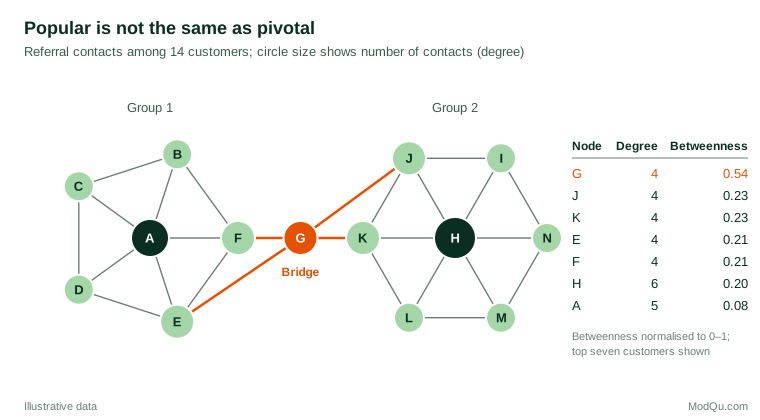
The two measures support different decisions. To reach many people directly, a hub such as H is valuable. To carry a message between the groups, or to judge what a lost connection would cost, G is the critical customer. Losing G would split the network into two disconnected parts.
Brokers, bridges and weak ties
The pattern in Figure 1 has a long history in social science. Granovetter (1973) argued that weak ties, such as acquaintances, often act as bridges between otherwise separate groups, and therefore carry new information that close friends, who know the same people, cannot. In his study of people who found jobs through personal contacts, most had heard about the job from someone they saw only occasionally or rarely.
Burt (2004) extended the idea with the concept of structural holes: gaps between groups that are not otherwise connected. In a study of managers in a large electronics company, those whose networks spanned such gaps were more likely to have their ideas judged valuable. For organisations, this suggests that people who connect departments, regions or customer segments are a source of innovation and also a point of vulnerability.
Whole-network structure
Beyond individual positions, analysts describe the network as a whole. Three measures are basic:
- Density is the share of possible links that are present. The network in Figure 1 has a density of 0.29.
- Average path length is the mean number of steps between pairs of nodes (2.6 in Figure 1).
- Clustering measures how often two contacts of the same node are also linked to each other, that is, how many triangles there are (0.56 on average in Figure 1).
Watts and Strogatz (1998) showed that many real networks, from film actor collaborations to the western United States power grid, are small worlds: they are highly clustered, like a lattice of local groups, yet have short average paths, like a random network. A few long-range links are enough to make a large network small, which helps explain why information, rumours and infections can spread quickly.
Hubs and degree distributions
Real networks also tend to have very unequal degree distributions. Barabási and Albert (1999) proposed that two mechanisms, growth and preferential attachment, in which new nodes are more likely to link to nodes that are already well connected, generate networks with a few very large hubs and a long, heavy tail of degrees. Figure 2 compares two simulated networks with the same number of nodes and links. When links form at random, no node has more than 12 links. When they form by preferential attachment, the largest hub has 149 links and 30 nodes have 20 or more.
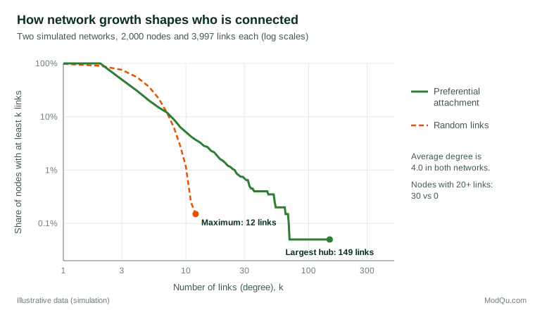
Such networks are often called scale-free, because their degree distribution approximately follows a power law. The label should be used with care. Broido and Clauset (2019) tested nearly 1,000 real networks and found that strongly scale-free structure is rare; many networks are heavy-tailed without following a power law closely. The practical lesson is that averages describe networks poorly: a few highly connected customers or suppliers can matter far more than the typical one.
Finding communities
Many networks contain communities, groups of nodes that are densely linked internally and sparsely linked to the rest. In customer data, communities may correspond to friendship circles, professional groups or segments with shared tastes. Detecting them is a form of cluster analysis that uses ties rather than attributes.
Girvan and Newman (2002) proposed finding communities by repeatedly removing the links with the highest betweenness, which are most likely to run between groups. Newman and Girvan (2004) then introduced modularity, a score for how much more densely connected the proposed groups are than would be expected by chance:
Q = Σc [ Lc ÷ m − (dc ÷ 2m)2 ]
where m is the total number of links, Lc is the number of links inside community c, and dc is the sum of the degrees of its nodes. In Figure 1, splitting the network into its two visible groups, with G counted in the first, gives Q ≈ 0.42. Newman and Girvan (2004) report that networks with clear community structure typically score between about 0.3 and 0.7. Fast algorithms that search for high-modularity partitions, such as the Louvain method, can handle very large networks; Blondel et al. (2008) applied theirs to a mobile phone network of 2.6 million customers. Fortunato (2010) reviews the many methods available and their limits, including the fact that modularity can miss small communities in large networks.
Statistical models for networks
Descriptive measures say what a network looks like; statistical models ask which processes could have produced it. The central difficulty is dependence: whether two people are linked depends on whether they share friends, which violates the independence assumptions of ordinary regression.
Two families of models address this. Stochastic block models assume that nodes belong to latent groups and that the probability of a link depends on the groups of the two nodes (Holland et al., 1983). They provide a model-based, probabilistic alternative to community detection. Exponential random graph models (ERGMs) treat the whole network as one observation and estimate how strongly local configurations such as mutual ties, shared partners and triangles shape it, while controlling for node attributes (Robins et al., 2007). They make it possible to ask, for example, whether employees are more likely to seek advice from colleagues in the same department after accounting for the general tendency of advice ties to form triangles.
Influence, homophily and causation
Network data invite causal stories: a customer bought because a friend did. Some of the most cited evidence comes from health research. Christakis and Fowler (2007) followed 12,067 people from 1971 to 2003 and reported that a person's chance of becoming obese increased by 57% if a friend became obese.
Such findings are hard to interpret. People tend to form ties with others who are like them, a pattern known as homophily that McPherson et al. (2001) document across race, age, religion, education, occupation and gender. Similar people may then change in similar ways because they share unobserved traits or environments, not because they influence each other. Shalizi and Thomas (2011) showed that, in observational network data, contagion and homophily based on unobserved characteristics are generically confounded: without further assumptions or an experiment, the data cannot separate them. Claims that one customer's behaviour causes another's therefore need designs such as randomised referral incentives, not only correlations between connected people.
Practical guidance for survey and business data
- Define the boundary first. Decide which people, firms or products count as nodes and which relationships count as ties, and record the rule. Network measures are only meaningful relative to that boundary.
- Design name generators carefully. Ask about a specific relationship and time frame, avoid tight caps on the number of names, and consider how recall and social desirability may shape answers (Marsden, 1990).
- Treat missing ties as a design problem. Non-respondents still have ties; ignoring them can bias centrality and density measures (Kossinets, 2006). Report response rates for network items separately.
- Match the measure to the question. Use degree for direct reach, betweenness for brokerage and vulnerability, eigenvector measures for influence through well-connected contacts, and community detection for segmentation.
- Use network-aware inference. Standard errors that treat linked observations as independent are too small. Permutation tests, ERGMs or block models are safer for testing hypotheses about ties.
- Protect privacy. Network data reveal information about people who never responded, so anonymise ties before sharing results.
Common mistakes
- Confusing popularity with importance. As Figure 1 shows, the most connected node is not always the most strategically placed.
- Over-interpreting power laws. A straight-looking line on a log-log plot is weak evidence; formal tests often reject a pure power law (Broido & Clauset, 2019).
- Treating communities as fixed truths. Different algorithms and resolutions can give different partitions. Check stability and interpret groups in light of what is known about the members.
- Reading influence into correlation. Similar behaviour among connected people may reflect homophily or shared environments rather than contagion (Shalizi & Thomas, 2011).
Key takeaways
Network analysis treats connections as data. Centrality measures show who is reachable, who brokers between groups and whose ties carry the most weight; whole-network measures reveal small-world structure, hubs and communities; and statistical models make it possible to test which processes shape a network. Its conclusions are only as good as the boundary and completeness of the data, and connection alone does not prove influence. Used with care, it reveals structure in markets and organisations that individual-level analysis cannot.
References
Barabási, A.-L., & Albert, R. (1999). Emergence of scaling in random networks. Science, 286(5439), 509–512. https://doi.org/10.1126/science.286.5439.509
Blondel, V. D., Guillaume, J.-L., Lambiotte, R., & Lefebvre, E. (2008). Fast unfolding of communities in large networks. Journal of Statistical Mechanics: Theory and Experiment, 2008(10), Article P10008. https://doi.org/10.1088/1742-5468/2008/10/P10008
Brin, S., & Page, L. (1998). The anatomy of a large-scale hypertextual Web search engine. Computer Networks and ISDN Systems, 30(1–7), 107–117. https://doi.org/10.1016/S0169-7552(98)00110-X
Broido, A. D., & Clauset, A. (2019). Scale-free networks are rare. Nature Communications, 10, Article 1017. https://doi.org/10.1038/s41467-019-08746-5
Burt, R. S. (2004). Structural holes and good ideas. American Journal of Sociology, 110(2), 349–399. https://doi.org/10.1086/421787
Christakis, N. A., & Fowler, J. H. (2007). The spread of obesity in a large social network over 32 years. New England Journal of Medicine, 357(4), 370–379. https://doi.org/10.1056/NEJMsa066082
Fortunato, S. (2010). Community detection in graphs. Physics Reports, 486(3–5), 75–174. https://doi.org/10.1016/j.physrep.2009.11.002
Freeman, L. C. (1978). Centrality in social networks conceptual clarification. Social Networks, 1(3), 215–239. https://doi.org/10.1016/0378-8733(78)90021-7
Girvan, M., & Newman, M. E. J. (2002). Community structure in social and biological networks. Proceedings of the National Academy of Sciences, 99(12), 7821–7826. https://doi.org/10.1073/pnas.122653799
Granovetter, M. S. (1973). The strength of weak ties. American Journal of Sociology, 78(6), 1360–1380. https://doi.org/10.1086/225469
Holland, P. W., Laskey, K. B., & Leinhardt, S. (1983). Stochastic blockmodels: First steps. Social Networks, 5(2), 109–137. https://doi.org/10.1016/0378-8733(83)90021-7
Kossinets, G. (2006). Effects of missing data in social networks. Social Networks, 28(3), 247–268. https://doi.org/10.1016/j.socnet.2005.07.002
Marsden, P. V. (1990). Network data and measurement. Annual Review of Sociology, 16, 435–463. https://doi.org/10.1146/annurev.so.16.080190.002251
McPherson, M., Smith-Lovin, L., & Cook, J. M. (2001). Birds of a feather: Homophily in social networks. Annual Review of Sociology, 27, 415–444. https://doi.org/10.1146/annurev.soc.27.1.415
Newman, M. E. J. (2003). The structure and function of complex networks. SIAM Review, 45(2), 167–256. https://doi.org/10.1137/S003614450342480
Newman, M. E. J., & Girvan, M. (2004). Finding and evaluating community structure in networks. Physical Review E, 69(2), Article 026113. https://doi.org/10.1103/PhysRevE.69.026113
Robins, G., Pattison, P., Kalish, Y., & Lusher, D. (2007). An introduction to exponential random graph (p*) models for social networks. Social Networks, 29(2), 173–191. https://doi.org/10.1016/j.socnet.2006.08.002
Shalizi, C. R., & Thomas, A. C. (2011). Homophily and contagion are generically confounded in observational social network studies. Sociological Methods & Research, 40(2), 211–239. https://doi.org/10.1177/0049124111404820
Wasserman, S., & Faust, K. (1994). Social network analysis: Methods and applications. Cambridge University Press. https://doi.org/10.1017/CBO9780511815478
Watts, D. J., & Strogatz, S. H. (1998). Collective dynamics of 'small-world' networks. Nature, 393(6684), 440–442. https://doi.org/10.1038/30918