
Statistics · Causal inference
Directed Acyclic Graphs for Causal Reasoning
How directed acyclic graphs turn assumptions about cause and effect into a simple diagram that shows which variables to adjust for, and which to leave alone, in business and survey analysis.
Every analysis that aims to estimate a causal effect from observational data rests on assumptions about how the variables influence one another. A directed acyclic graph (DAG) writes those assumptions down as a picture. Each variable is a node, and an arrow from one node to another means "may directly cause". The graph is directed because arrows have a direction, and acyclic because no variable can cause itself through a loop. Developed in computer science and statistics (Pearl, 2009) and brought into epidemiology by Greenland et al. (1999), DAGs are now a standard tool for deciding which variables a regression should include.
Three basic structures
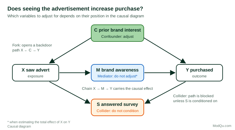
Almost everything about DAGs follows from three patterns of three variables, illustrated in Figure 1 with a question a marketing team might ask: does seeing an advertisement (X) increase purchase (Y)?
- Confounder (fork): X ← C → Y. Prior interest in the brand makes people more likely both to notice the advertisement and to buy. The fork opens a non-causal "backdoor" path between X and Y, so the confounder should be adjusted for.
- Mediator (chain): X → M → Y. The advertisement raises brand awareness, which in turn raises purchase. Adjusting for the mediator blocks part of the very effect we want, so it should not be adjusted for when estimating the total effect.
- Collider: X → S ← Y. Both exposure and purchase make a customer more likely to answer a follow-up survey. A collider blocks the path by default; conditioning on it, for example by analysing only survey respondents, opens a spurious association.
The backdoor criterion
The DAG turns the choice of control variables into a set of rules. A path between X and Y is blocked if it passes through a non-collider that is adjusted for, or through a collider that is not adjusted for (and none of whose descendants is adjusted for). Pearl's backdoor criterion states that a set of variables is sufficient to estimate the effect of X on Y if it blocks every path from X to Y that begins with an arrow into X, and contains no descendant of X (Pearl, 2009). In Figure 1, the set {C} meets the criterion; adding M or S would break it.
This replaces the common habit of "controlling for everything available". Rohrer (2018) shows, with examples from psychology, how adjusting for the wrong variable can create or hide associations, and Elwert and Winship (2014) explain how conditioning on a collider, including through sample selection, produces bias.
Why DAGs matter for survey data
Survey analysts meet colliders more often than they realise. Selection into a sample, into a panel or into a set of completed interviews is a form of conditioning. If both the exposure and the outcome affect who responds, the respondents are a conditioned sample, and a relationship can appear among them that does not exist in the population (Hernán et al., 2004). Drawing the DAG, with a node for response, makes the risk visible and points to remedies such as weighting on the causes of response.
DAGs also help with reporting. Westreich and Greenland (2013) describe the "Table 2 fallacy": presenting every coefficient from a multiple regression as if each were a causal effect. A model adjusted correctly for the effect of X on Y does not, in general, give valid causal estimates for the covariates, because each would require its own adjustment set.
Practical guidance
- Draw the graph before looking at the data. Use subject knowledge, the timing of measurement and the survey design to decide which arrows to include.
- Missing arrows are the strong assumptions. Every absent arrow claims that no direct effect exists. Make those claims deliberately.
- Include unmeasured variables. Show them as nodes; if one opens a backdoor path you cannot block, no adjustment will remove the bias, and a design such as an experiment or an instrumental variable may be needed.
- Use software for larger graphs. The free tool DAGitty finds adjustment sets and lists the testable implications of a graph (Textor et al., 2016).
- Publish the graph. Tennant et al. (2021) review the use of DAGs in applied health research and recommend reporting the full diagram and explaining how the adjustment set was derived from it.
Limitations
A DAG is only as good as the knowledge behind it. It shows qualitative assumptions, not the size or shape of effects, and different experts may draw different graphs. Its value is that it makes those disagreements explicit and checkable, rather than leaving them hidden in a list of control variables.
Key takeaways
Directed acyclic graphs make causal assumptions visible. Adjust for confounders, leave mediators alone when estimating total effects, and never condition on colliders, including through sample selection. Use the backdoor criterion to choose control variables, and report the graph alongside the results.
References
Elwert, F., & Winship, C. (2014). Endogenous selection bias: The problem of conditioning on a collider variable. Annual Review of Sociology, 40, 31–53. https://doi.org/10.1146/annurev-soc-071913-043455
Greenland, S., Pearl, J., & Robins, J. M. (1999). Causal diagrams for epidemiologic research. Epidemiology, 10(1), 37–48. https://doi.org/10.1097/00001648-199901000-00008
Hernán, M. A., Hernández-Díaz, S., & Robins, J. M. (2004). A structural approach to selection bias. Epidemiology, 15(5), 615–625. https://doi.org/10.1097/01.ede.0000135174.63482.43
Pearl, J. (2009). Causality: Models, reasoning, and inference (2nd ed.). Cambridge University Press. https://doi.org/10.1017/CBO9780511803161
Rohrer, J. M. (2018). Thinking clearly about correlations and causation: Graphical causal models for observational data. Advances in Methods and Practices in Psychological Science, 1(1), 27–42. https://doi.org/10.1177/2515245917745629
Tennant, P. W. G., Murray, E. J., Arnold, K. F., Berrie, L., Fox, M. P., Gadd, S. C., Harrison, W. J., Keeble, C., Ranker, L. R., Textor, J., Tomova, G. D., Gilthorpe, M. S., & Ellison, G. T. H. (2021). Use of directed acyclic graphs (DAGs) to identify confounders in applied health research: Review and recommendations. International Journal of Epidemiology, 50(2), 620–632. https://doi.org/10.1093/ije/dyaa213
Textor, J., van der Zander, B., Gilthorpe, M. S., Liśkiewicz, M., & Ellison, G. T. H. (2016). Robust causal inference using directed acyclic graphs: The R package 'dagitty'. International Journal of Epidemiology, 45(6), 1887–1894. https://doi.org/10.1093/ije/dyw341
Westreich, D., & Greenland, S. (2013). The Table 2 fallacy: Presenting and interpreting confounder and modifier coefficients. American Journal of Epidemiology, 177(4), 292–298. https://doi.org/10.1093/aje/kws412