
Statistics · Causal inference
Difference-in-Differences Analysis
How difference-in-differences compares changes over time in treated and untreated groups to estimate causal effects, why parallel trends matter, and what recent research says about staggered roll-outs.
A company launches an advertising campaign in some regions but not others. A city introduces a sugar tax while its neighbours do not. A retailer redesigns its stores in one province first. In each case, someone wants to know what the change achieved. A simple before-and-after comparison in the affected area is tempting, but it mixes the effect of the change with everything else that happened at the same time: seasonal patterns, the economy, competitors' moves, news events. A simple comparison between affected and unaffected areas after the change is no better, because the areas may have differed long before.
Difference-in-differences (often shortened to DiD or diff-in-diff) combines the two comparisons. It measures how much the treated group changed over time, measures how much a comparison group changed over the same period, and attributes the difference between those two changes to the treatment. It is one of the most widely used designs for evaluating policies, programmes and business interventions from observational data, and the approach has a long history in both epidemiology and economics (Angrist & Pischke, 2009; Lechner, 2011).
The basic idea
Causal questions are about potential outcomes: what happened to the treated group, and what would have happened to the same group without the treatment (Rubin, 1974; Holland, 1986). The second quantity, the counterfactual, is never observed. Difference-in-differences estimates it by assuming that, without treatment, the treated group would have followed the same trend as the comparison group.
With two groups and two periods, the estimator is simply:
DiD = (ȲT,post − ȲT,pre) − (ȲC,post − ȲC,pre)
Here Ȳ is the average outcome, T is the treated group and C the comparison (control) group. The first bracket removes stable differences between the groups; the second removes changes over time that affect both groups equally. What remains is the change in the treated group that the comparison group's experience cannot explain.
The most famous application is Card and Krueger's (1994) study of the minimum wage. When New Jersey raised its minimum wage in 1992, they surveyed fast-food restaurants in New Jersey and in neighbouring eastern Pennsylvania, where the minimum did not change, before and after the increase. Comparing the change in employment in New Jersey with the change in Pennsylvania, they found no evidence that the higher minimum wage reduced employment, a result that challenged a common prediction of economic theory and helped make the design central to applied economics. Card (1990) had earlier used the same logic to study how the sudden arrival of migrants in Miami during the 1980 Mariel boatlift affected local workers, comparing Miami with similar cities. Both studies are natural experiments: the researchers did not assign the treatment, but an outside event created a credible comparison.
A worked example
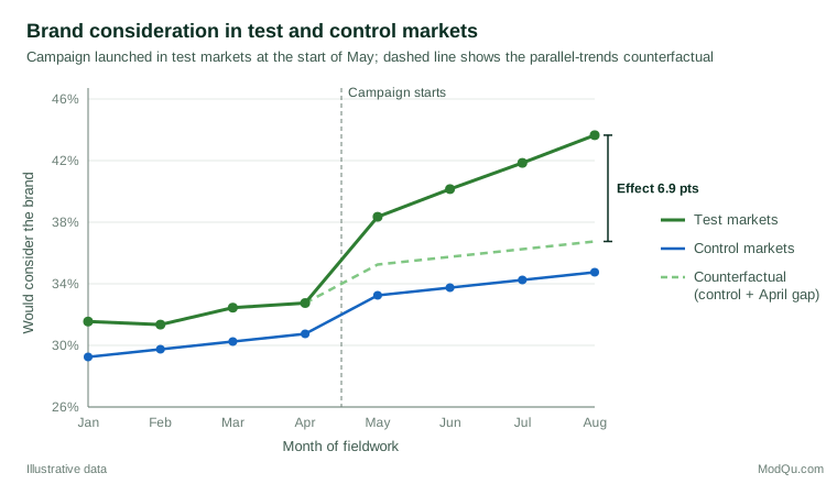
Consider a hypothetical consumer brand that runs a television and online campaign in 12 test markets from the start of May, while 20 similar markets see no campaign. A monthly brand tracker interviews about 500 adults per market and asks whether they would consider buying the brand. Table 1 summarises the four months before and the four months after launch.
| Hypothetical tracker results | Jan–Apr (pre) | May–Aug (post) | Change |
|---|---|---|---|
| Test markets | 32.0% | 41.0% | +9.0 |
| Control markets | 30.0% | 34.0% | +4.0 |
| Difference-in-differences | +5.0 |
A simple before-and-after comparison in the test markets would credit the campaign with 9 points. But consideration also rose by 4 points in markets with no campaign, perhaps because of a seasonal lift or a category-wide news story. The difference-in-differences estimate of the campaign's effect is 9 − 4 = 5 percentage points. Equally, comparing test and control markets after launch would suggest an 11-point effect, ignoring the fact that the test markets were already 2 points ahead before the campaign.
Figure 1 shows the monthly data behind the table. The test markets run roughly parallel to the control markets until April, then pull away. The dashed line is the counterfactual implied by the design: the control markets' path shifted up by the pre-launch gap.
The regression formulation
The same estimate can be obtained from a regression, which makes it easy to add covariates and compute standard errors:
Yit = β0 + β1Treati + β2Postt + β3(Treati × Postt) + εit
Treat is 1 for units in the treated group, Post is 1 for periods after the intervention, and the coefficient β3 on the interaction is the difference-in-differences estimate. With many units and periods, the group and time indicators are usually replaced by unit and period fixed effects, giving the two-way fixed effects model:
Yit = αi + λt + δDit + εit
Here αi absorbs everything stable about each unit, λt absorbs everything that affects all units in a given period, and Dit indicates whether unit i is treated at time t. When all treated units start treatment at the same time, δ equals the simple difference-in-differences. Angrist and Pischke (2009) and Imbens and Wooldridge (2009) give clear treatments of this framework.
The estimand is the average treatment effect on the treated (ATT): the effect of the campaign in the markets that received it. It does not automatically tell you what would happen if the campaign were rolled out to different markets.
The parallel trends assumption
Everything rests on one assumption: in the absence of treatment, the average outcome in the treated group would have changed by the same amount as in the comparison group. This is the parallel trends assumption. It does not require the groups to have the same level, only the same change. It cannot be tested directly, because the treated group's untreated path after launch is never observed.
Several situations commonly break it:
- Selection on shocks. Treatment is often targeted at places or people that are doing unusually badly or well. Ashenfelter and Card (1985) found that participants in a training programme had a dip in earnings just before they enrolled, so their later recovery would have happened anyway and a naive comparison overstates the programme's effect. A business that launches a campaign in its weakest regions faces the same risk.
- Different underlying trends. Fast-growing regions or segments may keep growing faster regardless of any intervention.
- Other changes at the same time. If a competitor exits only the test markets during the campaign, the design will attribute that change to the campaign.
- Anticipation. If customers or staff change their behaviour before the official start, because the change was announced in advance, the pre-period is already contaminated.
The assumption also depends on the scale of measurement. Trends that are parallel in percentages may not be parallel in logarithms or odds. Athey and Imbens (2006) developed a "changes-in-changes" model that relaxes this dependence and allows effects to vary across the outcome distribution.
Conditional parallel trends
Sometimes trends are plausibly parallel only after accounting for differences between the groups, for example in age mix or urban share. Abadie (2005) showed how to estimate difference-in-differences when parallel trends hold conditional on covariates, by reweighting the comparison group using the propensity score. Sant'Anna and Zhao (2020) combined this reweighting with outcome regression in doubly robust estimators, which remain consistent if either the propensity score model or the outcome model is correctly specified. Covariates used in this way should be measured before treatment, because variables affected by the treatment can bias the estimate.
Checking the assumption with event studies
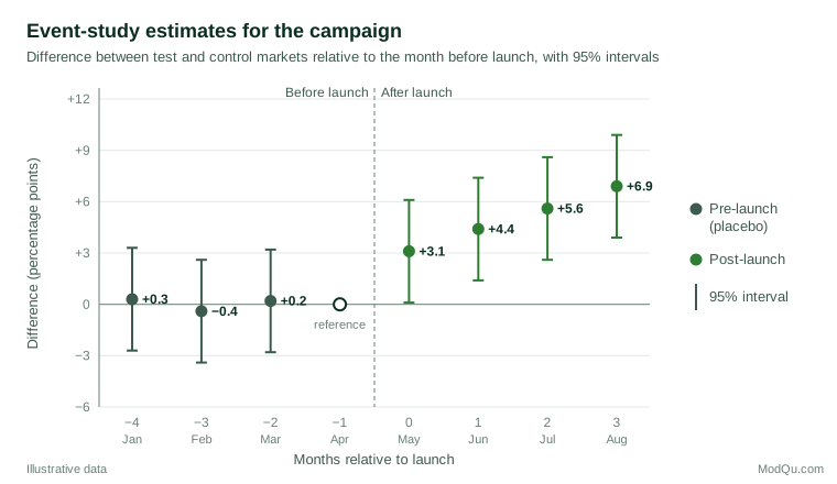
Although parallel trends cannot be proved, its plausibility can be examined when several pre-treatment periods are available. The standard tool is an event study: a regression that estimates a separate treated-versus-control difference for each period before and after the intervention, relative to a reference period (usually the last period before treatment).
Figure 2 shows an event study for the hypothetical campaign. The estimates for January to March are close to zero and their 95% intervals include zero, which is what we would expect if the groups were moving in parallel before launch. After launch, the estimates rise from 3.1 points in the first month to 6.9 points in the fourth, suggesting an effect that builds over time. The average of the four post-launch estimates is 5.0 points, matching Table 1.
The event study also changes the business message. A single 5-point average hides the fact that the effect was still growing when the data ended. If the campaign had stopped in August, a manager would want to know whether the gain persists or fades, and further waves of the tracker for both groups would answer that question directly.
Pre-trend checks need careful reading. A flat pre-period is reassuring but not proof: trends can diverge exactly when treatment starts for reasons unrelated to it. Roth (2022) showed that conventional pre-tests often have low power to detect meaningful violations, and that analysing only studies that pass such a test can make the bias of the surviving estimates worse. Rambachan and Roth (2023) proposed a more credible approach: instead of asking whether pre-trends are zero, ask how large a violation of parallel trends after treatment would have to be, relative to the variation seen before treatment, to overturn the conclusion. Reporting this kind of sensitivity analysis alongside the event study is increasingly regarded as good practice (Roth et al., 2023).
Staggered roll-outs and the two-way fixed effects problem
Many business and policy changes are rolled out in waves: a new store format reaches some provinces in 2023, others in 2024 and the rest in 2025. For years the standard approach was to fit the two-way fixed effects model above, with Dit switching on when each unit was treated. A wave of research has shown that this can go seriously wrong when treatment effects differ across groups or change over time.
Goodman-Bacon (2021) showed that the two-way fixed effects estimate is a weighted average of all possible two-group, two-period comparisons in the data. Some of these comparisons use units that were treated earlier as the control group for units treated later. If the effect of the earlier treatment is still growing, those "controls" are moving for reasons that have nothing to do with the later treatment, and the comparison is contaminated. Work by de Chaisemartin and D'Haultfœuille (2020) showed that the estimate can place negative weights on some group-period effects, so that in extreme cases it could even have the opposite sign from every underlying effect. Sun and Abraham (2021) showed that the same problem affects event-study coefficients, which can pick up effects from other periods.
Several alternative estimators avoid these problems by making only "clean" comparisons, against units not yet treated or never treated:
- Callaway and Sant'Anna (2021) estimate a separate effect for each cohort (units first treated at the same time) in each period, then aggregate these into overall, cohort-specific or event-time summaries.
- Sun and Abraham (2021) propose an interaction-weighted event-study estimator with the same goal.
- Borusyak et al. (2024) propose an imputation approach: fit a model of untreated outcomes using only untreated observations, predict what treated units would have done without treatment, and average the differences.
Roth et al. (2023) provide a readable synthesis of this literature. The practical lesson is that when treatment timing varies, analysts should not rely on a single two-way fixed effects coefficient. They should use one of the heterogeneity-robust estimators, show which comparisons drive the estimate, and report effects by cohort and by time since treatment.
Inference: getting the uncertainty right
Difference-in-differences studies typically involve a small number of groups observed repeatedly, and outcomes within a group are correlated over time. Bertrand et al. (2004) showed the consequences. Applying placebo "laws" at random to American states in data where no real effect existed, they found that conventional standard errors rejected the null hypothesis far more often than the nominal 5%, because they ignored serial correlation within states. Their recommended remedies include clustering standard errors at the level at which treatment is assigned, and collapsing the data into pre- and post-period averages.
In the worked example, treatment is assigned to markets, so standard errors should be clustered by market, not computed as if the roughly 128,000 interviews collected over eight months were independent. Ignoring clustering, the hypothetical standard error of the 5.0-point estimate would be about 0.5 points; clustering by market raises it to about 1.2 points, giving a 95% interval of roughly 2.6 to 7.4 points. The conclusion survives, but with much less precision than the naive figure suggests.
Clustering itself works poorly when there are few clusters. Donald and Lang (2007) discuss inference with a small number of groups, Cameron et al. (2008) show that a wild cluster bootstrap gives more reliable tests when clusters are few, and Conley and Taber (2011) develop methods for the common case where only a handful of groups change policy. A study with one treated region and one control region has, in effect, a sample size of two for the purposes of inference, however many interviews it contains.
Extensions: adding a third difference
Sometimes a second comparison inside the treated area can strengthen the design. Suppose the campaign targeted adults under 35, and older adults in the same markets were barely exposed. Comparing the difference-in-differences for younger adults with the difference-in-differences for older adults gives a triple difference. It removes shocks that hit a whole market, such as a local store opening, as well as shocks that hit a whole age group nationally. The price is a new assumption: that without the campaign, the gap between younger and older adults would have evolved in the same way in test and control markets.
When there are few treated units: synthetic control
If only one market, region or country is treated, choosing a single comparison is fragile. The synthetic control method of Abadie et al. (2010) builds a weighted combination of untreated units that closely tracks the treated unit before the intervention, then uses that combination as the counterfactual afterwards. Their study of California's 1988 tobacco control programme, which compared California with a weighted combination of other states, is the standard illustration. Synthetic control is best viewed as a close relative of difference-in-differences that is useful when the parallel trends assumption is doubtful for any single comparison group.
Practical guidance for survey and business data
Difference-in-differences fits naturally with tracking studies, customer panels and sales data, but survey data bring particular challenges. Wing et al. (2018) offer a useful checklist for designing such studies.
- Keep measurement constant. A change in questionnaire wording, question order, fieldwork agency or survey mode at the same time as the intervention will be confounded with it. If the tracker changes, it should change in both groups at once, and ideally not at the moment of treatment.
- Know whether you have a panel or repeated cross-sections. A panel follows the same people, which improves precision and supports individual fixed effects. Repeated cross-sections draw new samples each wave, which is valid but requires the composition of each group's sample to be stable. If the profile of respondents in the test markets changes after launch, for example because the campaign changed who responds, the estimate can be biased (Lechner, 2011).
- Use consistent weighting. Apply the same weighting scheme in all waves and both groups, and use design-based or cluster-robust standard errors.
- Choose the comparison group before looking at outcomes. Picking control markets because they make the result look good undermines the analysis. Define the comparison group in a pre-registered plan where possible.
- Collect several pre-treatment periods. One pre-period allows a DiD estimate but no check on trends. Three or more allow an event study.
- Watch for spillovers. A national online campaign may reach consumers in "control" markets; shoppers may cross borders to buy. Spillovers violate the assumption that the control group is unaffected and usually bias the estimate towards zero.
- Plan the sample around groups, not just interviews. Precision depends heavily on the number of treated and control groups, so ten markets of 300 interviews usually beat two markets of 1,500.
Common mistakes
- Reporting a before-and-after change as an effect. Without a comparison group, any common shock is attributed to the intervention.
- Treating a non-significant pre-trend test as proof that parallel trends hold (Roth, 2022).
- Using a single two-way fixed effects coefficient with staggered timing when effects may vary across cohorts or over time (Goodman-Bacon, 2021).
- Ignoring clustering and serial correlation, which can make standard errors much too small (Bertrand et al., 2004).
- Adjusting for variables affected by the treatment, such as awareness measured after the campaign began.
- Forgetting the estimand. The result is the average effect in the groups that were treated, during the period studied, and it may not carry over to other groups or later periods.
Key takeaways
Difference-in-differences estimates the effect of an intervention by comparing the change in a treated group with the change in a comparison group over the same period. It removes stable differences between groups and shocks common to both, and it relies on a single core assumption: that without treatment, the two groups would have followed parallel trends. Plotting the data, estimating an event study and running sensitivity analyses for violations of parallel trends make that assumption visible. When treatment is rolled out in waves, modern heterogeneity-robust estimators should replace the traditional two-way fixed effects regression. Standard errors must reflect the number of groups, not the number of interviews. With these safeguards, difference-in-differences is one of the most useful tools available for turning tracking data into credible evidence about what an intervention actually achieved.
References
Abadie, A. (2005). Semiparametric difference-in-differences estimators. The Review of Economic Studies, 72(1), 1–19. https://doi.org/10.1111/0034-6527.00321
Abadie, A., Diamond, A., & Hainmueller, J. (2010). Synthetic control methods for comparative case studies: Estimating the effect of California's tobacco control program. Journal of the American Statistical Association, 105(490), 493–505. https://doi.org/10.1198/jasa.2009.ap08746
Angrist, J. D., & Pischke, J.-S. (2009). Mostly harmless econometrics: An empiricist's companion. Princeton University Press. https://doi.org/10.1515/9781400829828
Ashenfelter, O., & Card, D. (1985). Using the longitudinal structure of earnings to estimate the effect of training programs. The Review of Economics and Statistics, 67(4), 648–660. https://doi.org/10.2307/1924810
Athey, S., & Imbens, G. W. (2006). Identification and inference in nonlinear difference-in-differences models. Econometrica, 74(2), 431–497. https://doi.org/10.1111/j.1468-0262.2006.00668.x
Bertrand, M., Duflo, E., & Mullainathan, S. (2004). How much should we trust differences-in-differences estimates? The Quarterly Journal of Economics, 119(1), 249–275. https://doi.org/10.1162/003355304772839588
Borusyak, K., Jaravel, X., & Spiess, J. (2024). Revisiting event-study designs: Robust and efficient estimation. The Review of Economic Studies, 91(6), 3253–3285. https://doi.org/10.1093/restud/rdae007
Callaway, B., & Sant'Anna, P. H. C. (2021). Difference-in-differences with multiple time periods. Journal of Econometrics, 225(2), 200–230. https://doi.org/10.1016/j.jeconom.2020.12.001
Cameron, A. C., Gelbach, J. B., & Miller, D. L. (2008). Bootstrap-based improvements for inference with clustered errors. The Review of Economics and Statistics, 90(3), 414–427. https://doi.org/10.1162/rest.90.3.414
Card, D. (1990). The impact of the Mariel boatlift on the Miami labor market. ILR Review, 43(2), 245–257. https://doi.org/10.1177/001979399004300205
Card, D., & Krueger, A. B. (1994). Minimum wages and employment: A case study of the fast-food industry in New Jersey and Pennsylvania. The American Economic Review, 84(4), 772–793.
Conley, T. G., & Taber, C. R. (2011). Inference with "difference in differences" with a small number of policy changes. The Review of Economics and Statistics, 93(1), 113–125. https://doi.org/10.1162/REST_a_00049
de Chaisemartin, C., & D'Haultfœuille, X. (2020). Two-way fixed effects estimators with heterogeneous treatment effects. American Economic Review, 110(9), 2964–2996. https://doi.org/10.1257/aer.20181169
Donald, S. G., & Lang, K. (2007). Inference with difference-in-differences and other panel data. The Review of Economics and Statistics, 89(2), 221–233. https://doi.org/10.1162/rest.89.2.221
Goodman-Bacon, A. (2021). Difference-in-differences with variation in treatment timing. Journal of Econometrics, 225(2), 254–277. https://doi.org/10.1016/j.jeconom.2021.03.014
Holland, P. W. (1986). Statistics and causal inference. Journal of the American Statistical Association, 81(396), 945–960. https://doi.org/10.1080/01621459.1986.10478354
Imbens, G. W., & Wooldridge, J. M. (2009). Recent developments in the econometrics of program evaluation. Journal of Economic Literature, 47(1), 5–86. https://doi.org/10.1257/jel.47.1.5
Lechner, M. (2011). The estimation of causal effects by difference-in-difference methods. Foundations and Trends in Econometrics, 4(3), 165–224. https://doi.org/10.1561/0800000014
Rambachan, A., & Roth, J. (2023). A more credible approach to parallel trends. The Review of Economic Studies, 90(5), 2555–2591. https://doi.org/10.1093/restud/rdad018
Roth, J. (2022). Pretest with caution: Event-study estimates after testing for parallel trends. American Economic Review: Insights, 4(3), 305–322. https://doi.org/10.1257/aeri.20210236
Roth, J., Sant'Anna, P. H. C., Bilinski, A., & Poe, J. (2023). What's trending in difference-in-differences? A synthesis of the recent econometrics literature. Journal of Econometrics, 235(2), 2218–2244. https://doi.org/10.1016/j.jeconom.2023.03.008
Rubin, D. B. (1974). Estimating causal effects of treatments in randomized and nonrandomized studies. Journal of Educational Psychology, 66(5), 688–701. https://doi.org/10.1037/h0037350
Sant'Anna, P. H. C., & Zhao, J. (2020). Doubly robust difference-in-differences estimators. Journal of Econometrics, 219(1), 101–122. https://doi.org/10.1016/j.jeconom.2020.06.003
Sun, L., & Abraham, S. (2021). Estimating dynamic treatment effects in event studies with heterogeneous treatment effects. Journal of Econometrics, 225(2), 175–199. https://doi.org/10.1016/j.jeconom.2020.09.006
Wing, C., Simon, K., & Bello-Gomez, R. A. (2018). Designing difference in difference studies: Best practices for public health policy research. Annual Review of Public Health, 39, 453–469. https://doi.org/10.1146/annurev-publhealth-040617-013507