
Statistics · Tests and models
Correlation: Pearson, Spearman and Their Limits
How Pearson's and Spearman's correlation coefficients measure association, how to read and test them in survey data, and the outliers, curves, restricted ranges and other traps that mislead.
Correlation is probably the most quoted statistic in business analysis after the average. "Satisfaction is strongly correlated with renewal." "Spending moves with income." "Respondents who trust the brand also rate its value highly." Behind each of these sentences is usually a single number, the correlation coefficient, that summarises how closely two variables move together on a scale from −1 to +1.
That single number is useful, but it is also easy to over-read. A coefficient of 0.2 can be important or trivial; a coefficient of zero can hide a strong relationship; and a coefficient of 0.6 can be produced by one unusual respondent. This article explains the two coefficients analysts use most, Pearson's r and Spearman's ρ (rho), shows how they are calculated and tested, and sets out their main limits for survey and business data. Whether a correlation reflects cause and effect is a separate question, covered in our companion article on correlation and causation; here the focus is on measuring association well.
Where correlation comes from
The idea of correlation grew out of Francis Galton's work on heredity and body measurements in the 1880s. Having studied the heights of parents and their children, he realised that the strength of a relationship between two measurements could be summarised by a single index of "co-relation" (Stigler, 1986). Karl Pearson turned Galton's idea into the product-moment formula still used today, deriving it as part of his mathematical work on regression and inheritance (Pearson, 1896). Charles Spearman (1904), a psychologist, introduced a version based on ranks and also showed that measurement error weakens observed correlations, a point that remains central for survey scales. Maurice Kendall (1938) later proposed a second rank-based measure, Kendall's τ (tau), built on counting agreeing and disagreeing pairs.
The coefficients are unchanged, but analysts now compute hundreds at once on data that are skewed, bounded, ordinal or weighted. They still work, provided their assumptions and limits are kept in view.
Pearson's correlation coefficient
Pearson's r measures the strength and direction of a linear (straight-line) relationship between two numeric variables. For n pairs of observations (xi, yi) with means x̄ and ȳ, it is:
r = Σ(xi − x̄)(yi − ȳ) ÷ √[Σ(xi − x̄)² × Σ(yi − ȳ)²]
The numerator adds up the products of deviations from the means. When high values of x tend to pair with high values of y, most products are positive and r is positive; when high values of one pair with low values of the other, r is negative. Dividing by the spread of each variable removes the units, so r is the same whether spending is measured in dollars or thousands of dollars, and it always lies between −1 and +1.
Rodgers and Nicewander (1988) described thirteen equivalent ways of looking at the same coefficient. Three are especially helpful in practice:
- A standardised covariance. r is the covariance of the two variables after each has been converted to z-scores (subtracting the mean and dividing by the standard deviation).
- A standardised regression slope. If both variables are standardised, r is the slope of the regression line: a one standard deviation rise in x is associated with an r standard deviation change in y.
- Shared variance. r² is the proportion of variance in one variable that a straight line on the other can account for. An r of 0.3 corresponds to only 9% shared variance, which is a useful antidote to over-enthusiastic reporting.
The second interpretation also explains Galton's original observation of regression to the mean: unless the correlation is perfect, an extreme value on one variable is, on average, paired with a less extreme value on the other.
Spearman's rank correlation
Spearman's ρ asks a different question: do the two variables move in the same order? Each variable is replaced by its ranks (1 for the smallest value, 2 for the next, and so on, with tied values given the average of the ranks they share), and Pearson's formula is then applied to the ranks. When there are no ties, this simplifies to:
ρ = 1 − 6Σdi² ÷ [n(n² − 1)]
where di is the difference between the two ranks of respondent i. Spearman's coefficient equals +1 whenever y always rises as x rises, whether the rise is straight, curved or stepped. It therefore measures a monotonic relationship rather than a linear one. Because ranks cannot be stretched by extreme values, ρ is much less sensitive to outliers and skewed distributions than r.
Kendall's τ is a close relative. It compares every pair of respondents and counts whether they are ordered the same way on both variables (concordant) or the opposite way (discordant). Its value is usually smaller in magnitude than ρ for the same data, but it has a direct interpretation as the difference between the probability of concordance and the probability of discordance, and it behaves well with small samples and many ties (Kendall, 1938).
A worked example
Consider a hypothetical sample of eight customers who rated their satisfaction from 0 to 10 and whose purchases over the past year were taken from sales records. Customer H is a small business that buys far more often than any household.
| Customer | A | B | C | D | E | F | G | H |
|---|---|---|---|---|---|---|---|---|
| Satisfaction (0–10) | 3 | 5 | 6 | 6 | 7 | 8 | 9 | 10 |
| Purchases in year | 2 | 4 | 3 | 6 | 7 | 8 | 9 | 40 |
| Rank of satisfaction | 1 | 2 | 3.5 | 3.5 | 5 | 6 | 7 | 8 |
| Rank of purchases | 1 | 3 | 2 | 4 | 5 | 6 | 7 | 8 |
The ranks agree almost perfectly, and Spearman's coefficient is ρ = 0.96 (Kendall's τ = 0.91). Pearson's coefficient is lower, at r = 0.72, because customer H's 40 purchases sit far above the straight line suggested by the other seven customers. If H had made 10 purchases instead, still the highest value in the sample, Pearson's r would rise to 0.95 while Spearman's ρ would not change at all, because the ranks would be the same.
Neither coefficient is "right". Pearson's r answers the question "how well does a straight line describe these values?" and Spearman's ρ answers "how consistently does a higher rating go with more purchases?" The gap between them is itself informative: it signals that the relationship is not linear, or that a few extreme values carry a lot of weight.
When the two coefficients disagree
Figure 1 shows four hypothetical data sets of 40 respondents each. In panel A the relationship is close to a straight line with random scatter, and the two coefficients nearly agree (r = 0.70, ρ = 0.68). In panel B the relationship is curved but always rising, as with a response that accelerates; the ranks are almost perfectly ordered (ρ = 0.97) but a straight line fits less well (r = 0.82).
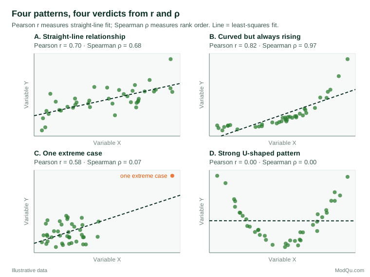
Panel C is the warning case. Thirty-nine respondents show no relationship at all, but one extreme case far from the cloud produces r = 0.58, a value most analysts would call substantial. Spearman's ρ stays near zero (0.07). In panel D, the relationship is strong but U-shaped, as can happen when both the cheapest and the most expensive options attract complaints. Both coefficients are zero, because neither measures non-monotonic patterns. Anscombe (1973) made the same point with four famous data sets that share the same correlation of 0.82 but look entirely different when plotted. The lesson is simple: always look at the scatterplot before reporting a coefficient.
Interpreting the size of a correlation
Cohen (1988) proposed rough benchmarks of 0.10, 0.30 and 0.50 for small, medium and large correlations in the behavioural sciences, while warning that such labels should only be used when no better basis for judgement exists. Later evidence suggests these benchmarks are optimistic. Reviewing hundreds of correlations published in individual differences research, Gignac and Szodorai (2016) found that the 25th, 50th and 75th percentiles were about 0.11, 0.19 and 0.29, and suggested 0.10, 0.20 and 0.30 as more realistic guides for small, typical and relatively large effects.
For business data, the best benchmark is usually context. A correlation of 0.15 between an advertising recall measure and later purchase may be commercially important across millions of customers; a correlation of 0.6 between two questions designed to measure the same attitude may be disappointingly low. It helps to translate the coefficient into practical terms, for example by showing the average outcome for respondents in the top and bottom quarters of the predictor, or by reporting the regression slope in natural units alongside r.
Testing and estimating a correlation
Significance tests
The usual test of whether a population correlation differs from zero uses the statistic t = r√(n − 2) ÷ √(1 − r²), compared with a t distribution on n − 2 degrees of freedom. With large samples, almost any non-zero correlation becomes statistically significant: with 2,000 respondents, r = 0.05 has a p-value below 0.05. Statistical significance therefore says little about whether a correlation matters. With small samples, the opposite problem arises, and quite large correlations may fail to reach significance.
The test also rests on assumptions. Fisher (1915) derived the exact sampling distribution of r for samples from a bivariate normal population, and this work underlies the usual tests and intervals. When the data are clearly non-normal, Bishara and Hittner (2012) found in simulations that the standard Pearson test could give too many false positives in some conditions, and that rank-based approaches such as Spearman's coefficient generally kept error rates closer to the nominal level.
Confidence intervals
A confidence interval is more informative than a test. Because the sampling distribution of r is skewed when the true correlation is not zero, the interval is calculated on a transformed scale, using Fisher's z transformation:
z = ½ ln[(1 + r) ÷ (1 − r)], with standard error 1 ÷ √(n − 3)
The interval is formed on the z scale and then converted back to the correlation scale. Figure 2 shows the result for an observed correlation of 0.30. With 25 respondents, the 95% interval runs from −0.11 to 0.62, so the data are consistent with no relationship and with a strong one. With 100 respondents it narrows to 0.11 to 0.47, and only with around 1,000 respondents does it shrink to 0.24 to 0.36.
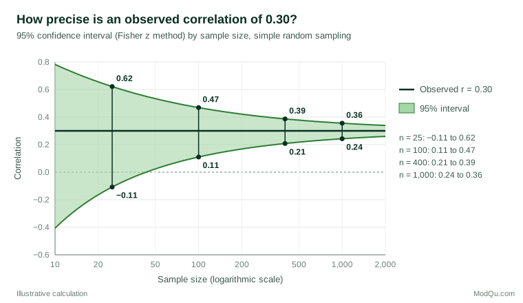
Correlations estimated from small samples are therefore much less stable than they look. Schönbrodt and Perugini (2013) used simulation to ask when a correlation estimate settles within a reasonable band around its true value, and concluded that in typical research scenarios the sample size should approach 250. Bonett and Wright (2000) give formulas for planning the sample size needed to estimate Pearson, Spearman and Kendall correlations with a chosen interval width. When the data are skewed or the coefficient is a rank correlation, a bootstrap interval, which resamples respondents many times and recomputes the coefficient each time, is a practical alternative (Efron & Tibshirani, 1994).
Choosing a coefficient for survey data
Survey data rarely look like the bivariate normal clouds of textbooks. Ratings are bounded, many questions have only five or seven categories, and spending, frequency and income variables are usually skewed. The following guidance covers most cases.
- Two continuous, roughly symmetric variables with a linear pattern: Pearson's r is efficient and easy to interpret.
- Skewed variables, outliers or a curved but consistently rising pattern: Spearman's ρ or Kendall's τ. In a large simulation and empirical comparison, de Winter et al. (2016) found that Pearson's r was slightly more precise for normally distributed data, but Spearman's ρ was preferable when distributions were heavy-tailed or contained outliers.
- Ordinal rating scales with few categories: Spearman's ρ or Kendall's τ (often τb, which adjusts for ties). When the categories are thought to reflect an underlying continuous attitude, a polychoric correlation estimates the correlation between those latent variables; Olsson (1979) set out the maximum likelihood method on which most software relies. Polychoric correlations are widely used as inputs to factor analysis of rating scales.
- Data with influential outliers that cannot simply be removed: robust coefficients, such as the percentage bend or winsorised correlation, limit the influence of extreme values while keeping more of the information than ranks (Wilcox, 2022).
- Weighted survey data: compute the coefficient with the survey weights, and use design-based methods or replicate weights for standard errors and intervals, because clustering and weighting usually widen intervals compared with a simple random sample (Lohr, 2021).
The limits of correlation
Only one kind of pattern
Pearson's r captures straight-line association, and Spearman's ρ captures monotonic association. Neither detects U-shaped, cyclical or threshold relationships, as panel D of Figure 1 shows. Newer measures try to capture any form of dependence: distance correlation is zero only when the variables are independent (Székely et al., 2007), and the maximal information coefficient was designed to rank many kinds of relationship in large data sets (Reshef et al., 2011). These are useful screening tools, but they are harder to interpret, and a plot is still the most reliable check.
Outliers and mixtures
A small number of extreme or unusual respondents can create, inflate, mask or reverse a correlation. So can mixing groups. If two customer segments differ in both average satisfaction and average spending, pooling them can produce a correlation that does not exist within either segment, or one in the opposite direction, which is the structure behind Simpson's paradox. Plot the data, check correlations within major segments, and report a rank or robust coefficient alongside Pearson's when results depend on a few cases.
Restricted range
A correlation depends on how much the variables vary in the sample. If a survey includes only current customers, or a validation study includes only applicants who were hired, the range of scores is narrower than in the full population and the correlation is usually weaker than it would otherwise be. Sackett and Yang (2000) describe the different ways in which range restriction arises and the corrections available for each. The reverse also happens: sampling only the extremes, such as very satisfied and very dissatisfied customers, inflates the correlation.
Measurement error
Survey measures contain random error. Spearman (1904) showed that unreliable measures pull correlations towards zero, a problem known as attenuation, and proposed a correction that divides the observed correlation by the square root of the product of the two measures' reliabilities. For example, an observed correlation of 0.40 between two scales with reliabilities of 0.70 and 0.80 corresponds to an estimated correlation of about 0.53 between the underlying constructs. The correction is useful for understanding constructs, but predictions in practice must use the measures actually available.
Aggregated data
Correlations computed on averages for regions, stores or time periods are often much stronger than the corresponding correlations between individuals. Robinson (1950) showed that correlations between proportions of census areas could differ greatly in size, and even in sign, from correlations among the people living in them. Using area-level correlations to make claims about individuals is the ecological fallacy. The same caution applies to correlations between brand-level averages in a tracking study.
Trends over time
Two series that both rise or fall over time will be correlated even if they have nothing to do with each other. Yule (1926) called these "nonsense correlations" and showed that a correlation of about 0.95 between two unrelated British time series was a product of their shared trends. For monthly sales, survey tracking scores and other time series, correlate changes rather than levels, or use models designed for time series.
Ratios and shared components
When two variables share a component, they will be correlated even if their other parts are unrelated. Pearson (1897) identified this "spurious correlation" for ratios with a common denominator. In business data, correlating revenue per customer with cost per customer, or one score with a total that includes it, creates correlation by construction.
Many correlations at once
A correlation matrix of 30 survey questions contains 435 distinct coefficients. Even if no true relationships existed, about 22 would be significant at the 5% level by chance. When many correlations are examined, use a correction such as the false discovery rate procedure of Benjamini and Hochberg (1995), and treat unexpected findings as hypotheses to confirm with new data.
Agreement is not correlation
Two measures can be highly correlated without agreeing. If one survey mode consistently produces ratings a point higher than another, their correlation can be close to 1 even though the scores never match. Bland and Altman (1986) showed why correlation is the wrong statistic for comparing two methods of measurement and proposed plotting the differences against the averages instead. The same logic applies when comparing two versions of a questionnaire or two panels.
Association is not causation
Finally, a correlation says nothing on its own about which variable affects the other, or whether a third factor drives both. Describe correlations as associations and avoid causal verbs such as "drives" unless the design supports them.
Common mistakes
- Reporting a coefficient without a plot. The four panels of Figure 1, and Anscombe's (1973) data sets, show how different data can share a coefficient.
- Reading r as a percentage. An r of 0.4 does not mean that 40% of the variation is explained; r² = 0.16 does.
- Concluding "no relationship" from r ≈ 0. A zero correlation rules out a linear relationship only.
- Treating a significant correlation as an important one. In large samples, trivial correlations are significant.
- Ignoring uncertainty in small samples. Report a confidence interval, especially for subgroups.
- Comparing correlations across samples with different spreads. Differences may reflect restricted range or different reliability rather than different relationships.
- Correlating averages and drawing conclusions about individuals.
Key takeaways
Correlation coefficients are compact and useful summaries of association, but each answers a narrow question. Pearson's r measures how well a straight line describes two numeric variables; Spearman's ρ and Kendall's τ measure how consistently they move in the same order and are more robust to outliers, skew and ordinal scales. Report the coefficient with a confidence interval, choose the version that suits the data, use survey weights where needed, and always look at the scatterplot. Above all, remember what a correlation cannot show: non-monotonic patterns, agreement between measures, individual-level relationships from aggregate data and, on its own, cause and effect. The coefficient is a starting point for analysis, not a conclusion.
References
Anscombe, F. J. (1973). Graphs in statistical analysis. The American Statistician, 27(1), 17–21. https://doi.org/10.1080/00031305.1973.10478966
Benjamini, Y., & Hochberg, Y. (1995). Controlling the false discovery rate: A practical and powerful approach to multiple testing. Journal of the Royal Statistical Society Series B: Statistical Methodology, 57(1), 289–300. https://doi.org/10.1111/j.2517-6161.1995.tb02031.x
Bishara, A. J., & Hittner, J. B. (2012). Testing the significance of a correlation with nonnormal data: Comparison of Pearson, Spearman, transformation, and resampling approaches. Psychological Methods, 17(3), 399–417. https://doi.org/10.1037/a0028087
Bland, J. M., & Altman, D. G. (1986). Statistical methods for assessing agreement between two methods of clinical measurement. The Lancet, 327(8476), 307–310. https://doi.org/10.1016/S0140-6736(86)90837-8
Bonett, D. G., & Wright, T. A. (2000). Sample size requirements for estimating Pearson, Kendall and Spearman correlations. Psychometrika, 65(1), 23–28. https://doi.org/10.1007/BF02294183
Cohen, J. (1988). Statistical power analysis for the behavioral sciences (2nd ed.). Routledge. https://doi.org/10.4324/9780203771587
de Winter, J. C. F., Gosling, S. D., & Potter, J. (2016). Comparing the Pearson and Spearman correlation coefficients across distributions and sample sizes: A tutorial using simulations and empirical data. Psychological Methods, 21(3), 273–290. https://doi.org/10.1037/met0000079
Efron, B., & Tibshirani, R. J. (1994). An introduction to the bootstrap. Chapman and Hall/CRC. https://doi.org/10.1201/9780429246593
Fisher, R. A. (1915). Frequency distribution of the values of the correlation coefficient in samples from an indefinitely large population. Biometrika, 10(4), 507–521. https://doi.org/10.2307/2331838
Gignac, G. E., & Szodorai, E. T. (2016). Effect size guidelines for individual differences researchers. Personality and Individual Differences, 102, 74–78. https://doi.org/10.1016/j.paid.2016.06.069
Kendall, M. G. (1938). A new measure of rank correlation. Biometrika, 30(1–2), 81–93. https://doi.org/10.1093/biomet/30.1-2.81
Lohr, S. L. (2021). Sampling: Design and analysis (3rd ed.). Chapman and Hall/CRC. https://doi.org/10.1201/9780429298899
Olsson, U. (1979). Maximum likelihood estimation of the polychoric correlation coefficient. Psychometrika, 44(4), 443–460. https://doi.org/10.1007/BF02296207
Pearson, K. (1896). Mathematical contributions to the theory of evolution. III. Regression, heredity, and panmixia. Philosophical Transactions of the Royal Society of London. Series A, 187, 253–318. https://doi.org/10.1098/rsta.1896.0007
Pearson, K. (1897). Mathematical contributions to the theory of evolution: On a form of spurious correlation which may arise when indices are used in the measurement of organs. Proceedings of the Royal Society of London, 60, 489–498. https://doi.org/10.1098/rspl.1896.0076
Reshef, D. N., Reshef, Y. A., Finucane, H. K., Grossman, S. R., McVean, G., Turnbaugh, P. J., Lander, E. S., Mitzenmacher, M., & Sabeti, P. C. (2011). Detecting novel associations in large data sets. Science, 334(6062), 1518–1524. https://doi.org/10.1126/science.1205438
Robinson, W. S. (1950). Ecological correlations and the behavior of individuals. American Sociological Review, 15(3), 351–357. https://doi.org/10.2307/2087176
Rodgers, J. L., & Nicewander, W. A. (1988). Thirteen ways to look at the correlation coefficient. The American Statistician, 42(1), 59–66. https://doi.org/10.1080/00031305.1988.10475524
Sackett, P. R., & Yang, H. (2000). Correction for range restriction: An expanded typology. Journal of Applied Psychology, 85(1), 112–118. https://doi.org/10.1037/0021-9010.85.1.112
Schönbrodt, F. D., & Perugini, M. (2013). At what sample size do correlations stabilize? Journal of Research in Personality, 47(5), 609–612. https://doi.org/10.1016/j.jrp.2013.05.009
Spearman, C. (1904). The proof and measurement of association between two things. The American Journal of Psychology, 15(1), 72–101. https://doi.org/10.2307/1412159
Stigler, S. M. (1986). The history of statistics: The measurement of uncertainty before 1900. Belknap Press of Harvard University Press.
Székely, G. J., Rizzo, M. L., & Bakirov, N. K. (2007). Measuring and testing dependence by correlation of distances. The Annals of Statistics, 35(6), 2769–2794. https://doi.org/10.1214/009053607000000505
Wilcox, R. R. (2022). Introduction to robust estimation and hypothesis testing (5th ed.). Elsevier. https://doi.org/10.1016/C2019-0-01225-3
Yule, G. U. (1926). Why do we sometimes get nonsense-correlations between time-series? A study in sampling and the nature of time-series. Journal of the Royal Statistical Society, 89(1), 1–63. https://doi.org/10.2307/2341482