
Statistics · Tests and models
Chi-Square Tests for Categorical Survey Data
How chi-square tests check whether survey answers differ between groups or match an expected pattern, how to read expected counts, residuals and Cramér's V, and how to adjust for weighted samples.
Most survey questions produce categories rather than numbers: preferred brand, region, age band, yes or no. When a cross-tabulation shows different percentages in different groups, the obvious question is whether the pattern reflects a real difference in the population or just sampling noise. The chi-square test, introduced by Pearson (1900), is the standard first answer. It compares the counts actually observed in a table with the counts we would expect if there were no relationship, and asks whether the gap is larger than chance would produce.
Two common versions
The goodness-of-fit test compares one categorical variable with a known or assumed distribution. For example, a researcher might check whether the regional mix of a sample matches census shares before weighting. Here the expected counts come from the assumed shares, and the degrees of freedom are the number of categories minus one, less any parameters estimated from the data.
The test of independence asks whether two categorical variables are related in the population, such as age group and preferred purchase channel. When the groups were sampled separately, the same calculation is called a test of homogeneity: do the groups share the same distribution of answers? Both versions use the same statistic:
χ² = Σ (O − E)² ÷ E
Here O is the observed count in each cell and E is the expected count. In a test of independence, the expected count for a cell is its row total multiplied by its column total, divided by the grand total. The degrees of freedom are (rows − 1) × (columns − 1), a result that Fisher (1922) established after earlier work had used the wrong value for contingency tables.
A worked example
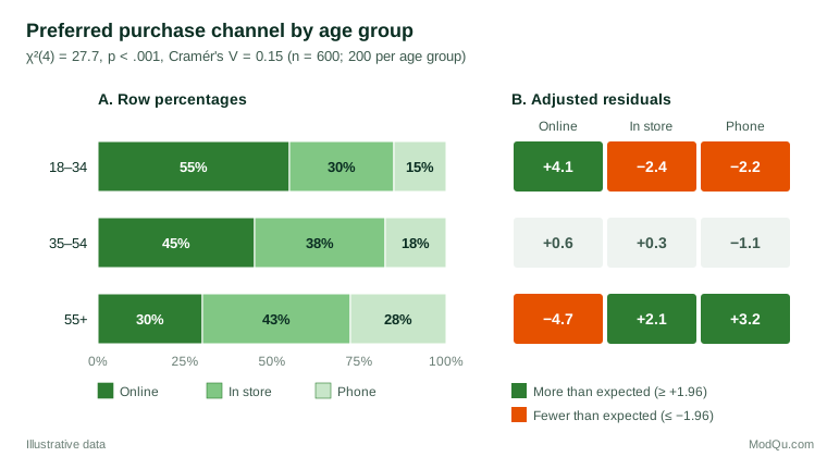
A hypothetical survey asks 600 respondents, 200 in each of three age groups, where they prefer to buy household goods. Online is chosen by 110 respondents aged 18–34, 90 aged 35–54 and 60 aged 55 and over. In total 260 choose online, 220 in store and 120 by phone. Because the age groups are equal in size, the expected count for online in every age group is 200 × 260 ÷ 600 = 86.7.
Adding up (O − E)² ÷ E over all nine cells gives χ² = 27.7 on (3 − 1) × (3 − 1) = 4 degrees of freedom, so p < .001. The 5% critical value for 4 degrees of freedom is 9.49, so the pattern is very unlikely under independence.
Going beyond the p-value
A significant chi-square says only that some association exists. Two further steps make the result useful.
Measure the strength. With large samples, even trivial differences become significant. Cramér's V, proposed by Cramér (1946), rescales chi-square to run from 0 (no association) to 1 (perfect association):
V = √(χ² ÷ (n × (k − 1)))
where k is the smaller of the number of rows and columns. In the example, V = √(27.7 ÷ (600 × 2)) = 0.15, a modest association. For a 2 × 2 table, V equals the absolute value of the phi coefficient.
Locate the pattern. Adjusted standardised residuals compare each observed count with its expected count on a scale that is approximately standard normal under independence (Haberman, 1973). Values beyond about ±2 mark cells that contribute strongly to the result. Figure 1 shows that younger respondents over-choose online (+4.1) and older respondents under-choose it (−4.7) while over-choosing phone (+3.2). With many cells, apply a stricter threshold, because some residuals will exceed ±2 by chance.
Assumptions and small samples
The chi-square test relies on a large-sample approximation. Cochran (1954) gave the familiar rule of thumb that no expected count should be below 1 and no more than about 20% of cells should have expected counts below 5. Note that the rule concerns expected counts, not observed ones. When it fails, merge sparse categories where this makes substantive sense, or use an exact test.
For 2 × 2 tables, Yates (1934) proposed a continuity correction, but it is now known to be overly conservative. After comparing the options by simulation, Campbell (2007) recommended an "N − 1" version of the chi-square test when every expected count is at least 1, and the Fisher–Irwin exact test otherwise.
The test also assumes that each respondent appears in exactly one cell. Delucchi (1983) lists violations of this rule among the most frequent misuses of the test. Two common survey cases break it:
- Multiple-response questions, where a respondent can tick several brands, so counts exceed the number of people.
- Paired data, such as the same people rating awareness before and after a campaign. Use McNemar's (1947) test for paired yes/no answers instead.
Weighted and complex survey samples
Standard chi-square tests assume simple random sampling. With weighting, stratification or clustering, the ordinary statistic no longer follows a chi-square distribution and is usually too large, which produces too many false positives. Rao and Scott (1981, 1984) developed corrections that rescale the statistic using estimated design effects. The simplest version divides chi-square by the average design effect. If the example came from a clustered sample with an average design effect of 1.8, the corrected statistic would be about 27.7 ÷ 1.8 = 15.4, with p = .004: still significant, but far less decisive. Modern survey software applies the fuller second-order correction automatically when the sample design is declared. Never run a chi-square test on weighted counts as though they were raw counts, because the inflated "sample size" makes p-values far too small.
Practical guidance
- Report the table with row or column percentages, the chi-square statistic, degrees of freedom, p-value, Cramér's V and the base sizes.
- Decide in advance which comparisons matter, and treat tests on many banner columns as exploratory.
- For ordered categories, such as satisfaction levels, a test for linear trend or an ordinal model uses the ordering and is usually more powerful than the general test (Agresti, 2013).
- For more than two variables, log-linear or logistic regression models extend the same logic and allow adjustment for confounders.
Common mistakes
- Treating a significant result as evidence of a strong or causal relationship.
- Applying the expected-count rule to observed counts.
- Testing percentages or weighted counts instead of correctly modelled counts.
- Ignoring paired or multiple-response structures.
- Reading single cells as significant without residuals or an adjustment for multiple comparisons.
Key takeaways
Chi-square tests are the workhorse for categorical survey data, testing whether answers are independent of group membership or fit an expected pattern. Use them with adequate expected counts, independent observations and corrections for complex samples. Always add Cramér's V to show strength and residuals to show where the difference lies, so that a significant result becomes an interpretable finding.
References
Agresti, A. (2013). Categorical data analysis (3rd ed.). Wiley.
Campbell, I. (2007). Chi-squared and Fisher–Irwin tests of two-by-two tables with small sample recommendations. Statistics in Medicine, 26(19), 3661–3675. https://doi.org/10.1002/sim.2832
Cochran, W. G. (1954). Some methods for strengthening the common χ² tests. Biometrics, 10(4), 417–451. https://doi.org/10.2307/3001616
Cramér, H. (1946). Mathematical methods of statistics. Princeton University Press. https://doi.org/10.1515/9781400883868
Delucchi, K. L. (1983). The use and misuse of chi-square: Lewis and Burke revisited. Psychological Bulletin, 94(1), 166–176. https://doi.org/10.1037/0033-2909.94.1.166
Fisher, R. A. (1922). On the interpretation of χ² from contingency tables, and the calculation of P. Journal of the Royal Statistical Society, 85(1), 87–94. https://doi.org/10.2307/2340521
Haberman, S. J. (1973). The analysis of residuals in cross-classified tables. Biometrics, 29(1), 205–220. https://doi.org/10.2307/2529686
McNemar, Q. (1947). Note on the sampling error of the difference between correlated proportions or percentages. Psychometrika, 12(2), 153–157. https://doi.org/10.1007/BF02295996
Pearson, K. (1900). On the criterion that a given system of deviations from the probable in the case of a correlated system of variables is such that it can be reasonably supposed to have arisen from random sampling. The London, Edinburgh, and Dublin Philosophical Magazine and Journal of Science, 50(302), 157–175. https://doi.org/10.1080/14786440009463897
Rao, J. N. K., & Scott, A. J. (1981). The analysis of categorical data from complex sample surveys: Chi-squared tests for goodness of fit and independence in two-way tables. Journal of the American Statistical Association, 76(374), 221–230. https://doi.org/10.1080/01621459.1981.10477633
Rao, J. N. K., & Scott, A. J. (1984). On chi-squared tests for multiway contingency tables with cell proportions estimated from survey data. The Annals of Statistics, 12(1), 46–60. https://doi.org/10.1214/aos/1176346391
Yates, F. (1934). Contingency tables involving small numbers and the χ² test. Journal of the Royal Statistical Society Series B: Statistical Methodology, 1(2), 217–235. https://doi.org/10.2307/2983604