
Statistics · Data science and machine learning
Bayesian Additive Regression Trees for Flexible Predictive Knowledge
How Bayesian additive regression trees combine many small decision trees with a Bayesian prior to give flexible predictions with honest uncertainty, and why they are popular for estimating varied treatment effects.
Predictive models face a familiar dilemma. Simple models, such as linear regression, are easy to interpret and come with standard errors, but they miss non-linear relationships and interactions unless the analyst specifies them in advance. Flexible machine learning methods, such as random forests and boosted trees, capture complex patterns automatically but usually give point predictions without a principled measure of uncertainty. Bayesian additive regression trees (BART), introduced by Chipman et al. (2010), sit between the two. BART builds a prediction from the sum of many small regression trees, as boosting does, but it treats the trees as unknown quantities in a Bayesian model with a prior that keeps each tree simple. The result is a method that adapts to complex data with little tuning and produces full posterior distributions for predictions and derived quantities.
From one tree to a sum of trees
A regression tree divides the predictor space into regions by a sequence of yes-or-no splits, such as "age under 35" or "more than three purchases last year", and predicts a constant value in each region. Single trees are easy to read but unstable and coarse: a small change in the data can change the splits, and a tree with a few leaves describes a smooth relationship as a staircase.
Ensembles of trees solve both problems. Random forests average many deep trees grown on resampled data (Breiman, 2001). Gradient boosting adds many shallow trees one at a time, each fitted to the errors of the current ensemble (Friedman, 2001), and fast implementations such as XGBoost have made it a standard tool (Chen & Guestrin, 2016). BART uses the same additive structure as boosting:
y = g(x; T1, M1) + g(x; T2, M2) + … + g(x; Tm, Mm) + ε, ε ~ N(0, σ2)
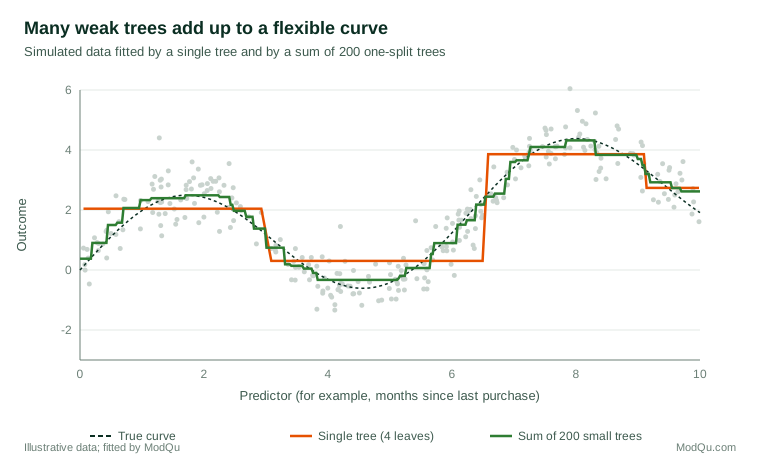
Here each g is a tree with structure Tj and leaf values Mj, and m is typically 50 to 200. Each tree contributes only a small part of the fit, so the sum can represent smooth curves and interactions that no single tree could capture (Figure 1).
The Bayesian ingredients
What makes BART distinctive is its prior, which acts as regularisation and keeps any single tree from dominating (Chipman et al., 2010).
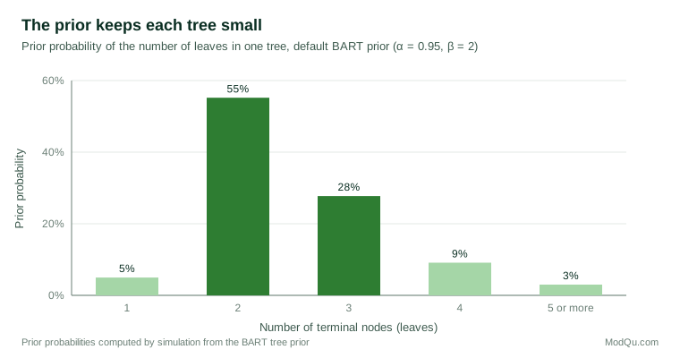
- Tree structure. Following the earlier Bayesian CART model (Chipman et al., 1998), a node at depth d splits with probability α(1 + d)−β. The default values α = 0.95 and β = 2 put most prior probability on trees with two or three leaves (Figure 2). Deep trees are possible but must be justified by the data.
- Leaf values. Leaf values are given a normal prior centred on zero and scaled so that the sum of all trees is likely to stay within the observed range of the outcome. With many trees, each leaf value is small, so each tree is a "weak learner".
- Error variance. An inverse chi-square prior is placed on σ2, calibrated to the residual variance of a simple regression.
The posterior is explored by a Markov chain Monte Carlo algorithm called Bayesian backfitting. At each step, one tree is updated given all the others: the algorithm proposes to grow, prune or change a split, accepts or rejects the proposal, and redraws the leaf values. Sweeping through all trees many times produces thousands of draws from the posterior distribution of the whole sum-of-trees function. Each draw gives a prediction for every case, so the spread of the draws gives uncertainty intervals for predictions, for differences between groups and for any other quantity computed from them (Gelman et al., 2013).
Why BART works well in practice
Several features explain BART's popularity (Hill et al., 2020).
- Little tuning. The default priors work well across a wide range of problems; cross-validation can refine them but is often unnecessary. This contrasts with boosting, which needs careful tuning of learning rate, tree depth and number of trees.
- Automatic non-linearity and interactions. Analysts do not need to specify which variables interact or how.
- Uncertainty quantification. Intervals come directly from the posterior. Their frequentist coverage is not guaranteed, but in many simulation studies it is reasonable.
- Theoretical support. Ročková and van der Pas (2020) showed that the BART posterior concentrates around the true function at near-optimal rates under suitable conditions, giving the method a firmer foundation.
- Extensions. Variants handle binary and categorical outcomes, counts (Murray, 2021), survival times and high-dimensional predictors with sparsity-inducing priors (Linero, 2018).
How BART compares with other tree ensembles
| Feature | Random forest | Gradient boosting | BART |
|---|---|---|---|
| How trees are combined | Average of many deep trees grown independently | Sum of shallow trees added one after another | Sum of shallow trees updated jointly by MCMC |
| Regularisation | Bootstrap samples and random feature choice | Learning rate, tree depth, number of trees | Prior on tree size and leaf values |
| Tuning needed | Little | Substantial | Little |
| Uncertainty | Indirect (for example, out-of-bag or jackknife methods) | Usually none without extra work | Posterior intervals for any quantity |
| Speed on large data | Fast | Very fast | Slower |
In predictive accuracy the three are often close, and a well-tuned boosting model may win on very large data sets. BART's advantage lies in combining competitive accuracy with uncertainty statements and stable results under default settings, which matter when the analysis must support decisions rather than only rank cases.
Choosing the number of trees
Chipman et al. (2010) recommend a default of 200 trees for prediction. Using fewer trees, say 20 to 50, makes each tree carry more of the fit and can make variable inclusion proportions more informative for variable selection, at some cost in predictive accuracy (Bleich et al., 2014). The choice rarely changes results much, and checking two settings is a sensible robustness test.
BART for causal inference and survey experiments
BART's best-known application is the estimation of causal effects. Hill (2011) proposed fitting BART to the outcome using both the treatment indicator and the covariates, then predicting each person's outcome under treatment and under control. The difference gives individual effect estimates, which can be averaged for the whole sample or for subgroups, each with posterior intervals. In a data analysis competition comparing many automated causal inference methods, BART-based approaches were among the best performers (Dorie et al., 2019).
Hahn et al. (2020) noted that plain BART can be biased when treatment assignment depends strongly on covariates, and proposed Bayesian causal forests, which model the outcome as a sum of a prognostic function and a separate treatment effect function with its own prior, often including an estimated propensity score as a predictor. This gives more reliable estimates of how effects vary across people.
For survey researchers, Green and Kern (2012) showed how BART can estimate heterogeneous treatment effects in survey experiments, such as question wording or framing experiments embedded in questionnaires. Rather than testing a few pre-chosen interactions, BART lets the data reveal which respondents react most strongly to a wording change, with uncertainty attached. Random-forest methods offer an alternative route to the same goal (Wager & Athey, 2018).
A worked example: who responds to a price message?
Consider a hypothetical online survey experiment with 4,000 respondents, half randomly shown a message about a price increase before being asked their purchase intention on a 0 to 10 scale. Covariates include age, income, current usage and attitudes to the brand.
A BART model of purchase intention on the treatment indicator and covariates estimates an average effect of the price message of −0.6 points, with a 95% posterior interval of −0.8 to −0.4. More usefully, the individual effect estimates vary widely. Summarising them with a simple tree fitted to the posterior means, an approach often used to interpret BART output, shows that the effect is about −1.3 points among light users with low brand attachment and close to zero among heavy users with strong attachment. Posterior intervals for these subgroup effects do not overlap. The business learns not only that the price message lowers intention, but where the loss is concentrated, and can tailor communication accordingly.
Interpreting BART
Because BART is a sum of many trees, it has no single set of coefficients. Interpretation relies on summaries:
- Partial dependence plots show how the predicted outcome changes with one variable, averaging over the others, with posterior bands.
- Variable inclusion proportions record how often each variable is used in splits across all trees and draws. Bleich et al. (2014) developed permutation-based tests from these proportions for variable selection.
- Subgroup summaries compare posterior predictions or effects for interpretable groups defined in advance or found by summarising the posterior.
Practical guidance
- Start with the defaults for the priors and number of trees, and run several chains to check that predictions agree.
- Check convergence by plotting the posterior draws of σ and of a few predictions; long burn-in periods are common with many predictors.
- Validate out of sample. Compare BART's accuracy and interval coverage with simpler models on held-out data before relying on it.
- Summarise for decision-makers with partial dependence plots, subgroup effects and intervals rather than raw posterior output.
- Combine with design. For causal questions, use BART within a sound design, such as a randomised experiment or a well-justified adjustment for confounders.
Software
BART is available in several well-maintained packages. The R package BART implements continuous, binary, count and survival versions with parallel computation (Sparapani et al., 2021), and bartMachine provides a Java-based implementation with tools for variable selection and interval estimation (Kapelner & Bleich, 2016).
Limitations and common mistakes
- Extrapolation. Like all tree methods, BART predicts constant values beyond the range of the data. Predictions for unusual combinations of predictors are weakly supported, although posterior intervals usually widen there.
- Computation. MCMC is slower than a single boosted model, though usually practical for tens of thousands of cases.
- Overconfidence in causal claims. BART can estimate effects only under the usual assumptions of no unmeasured confounding and overlap between groups; its flexibility does not remove the need for good design.
- Over-reading individual effects. Individual estimates are noisy; decisions should rest on subgroup patterns with clear posterior support.
Key takeaways
Bayesian additive regression trees combine the flexibility of tree ensembles with the uncertainty quantification of Bayesian inference. A sum of many small trees, held in check by a prior that favours simplicity, captures non-linear relationships and interactions with little tuning, and posterior draws give intervals for any quantity of interest. These properties make BART a strong default for flexible prediction and for estimating how effects vary across people, including in survey experiments, provided its outputs are interpreted with the same care as any other model.
References
Bleich, J., Kapelner, A., George, E. I., & Jensen, S. T. (2014). Variable selection for BART: An application to gene regulation. The Annals of Applied Statistics, 8(3), 1750–1781. https://doi.org/10.1214/14-AOAS755
Breiman, L. (2001). Random forests. Machine Learning, 45(1), 5–32. https://doi.org/10.1023/A:1010933404324
Chen, T., & Guestrin, C. (2016). XGBoost: A scalable tree boosting system. In Proceedings of the 22nd ACM SIGKDD International Conference on Knowledge Discovery and Data Mining (pp. 785–794). Association for Computing Machinery. https://doi.org/10.1145/2939672.2939785
Chipman, H. A., George, E. I., & McCulloch, R. E. (1998). Bayesian CART model search. Journal of the American Statistical Association, 93(443), 935–948. https://doi.org/10.1080/01621459.1998.10473750
Chipman, H. A., George, E. I., & McCulloch, R. E. (2010). BART: Bayesian additive regression trees. The Annals of Applied Statistics, 4(1), 266–298. https://doi.org/10.1214/09-AOAS285
Dorie, V., Hill, J., Shalit, U., Scott, M., & Cervone, D. (2019). Automated versus do-it-yourself methods for causal inference: Lessons learned from a data analysis competition. Statistical Science, 34(1), 43–68. https://doi.org/10.1214/18-STS667
Friedman, J. H. (2001). Greedy function approximation: A gradient boosting machine. The Annals of Statistics, 29(5), 1189–1232. https://doi.org/10.1214/aos/1013203451
Gelman, A., Carlin, J. B., Stern, H. S., Dunson, D. B., Vehtari, A., & Rubin, D. B. (2013). Bayesian data analysis (3rd ed.). Chapman and Hall/CRC. https://doi.org/10.1201/b16018
Green, D. P., & Kern, H. L. (2012). Modeling heterogeneous treatment effects in survey experiments with Bayesian additive regression trees. Public Opinion Quarterly, 76(3), 491–511. https://doi.org/10.1093/poq/nfs036
Hahn, P. R., Murray, J. S., & Carvalho, C. M. (2020). Bayesian regression tree models for causal inference: Regularization, confounding, and heterogeneous effects (with discussion). Bayesian Analysis, 15(3), 965–1056. https://doi.org/10.1214/19-BA1195
Hill, J. L. (2011). Bayesian nonparametric modeling for causal inference. Journal of Computational and Graphical Statistics, 20(1), 217–240. https://doi.org/10.1198/jcgs.2010.08162
Hill, J., Linero, A., & Murray, J. (2020). Bayesian additive regression trees: A review and look forward. Annual Review of Statistics and Its Application, 7, 251–278. https://doi.org/10.1146/annurev-statistics-031219-041110
Kapelner, A., & Bleich, J. (2016). bartMachine: Machine learning with Bayesian additive regression trees. Journal of Statistical Software, 70(4), 1–40. https://doi.org/10.18637/jss.v070.i04
Linero, A. R. (2018). Bayesian regression trees for high-dimensional prediction and variable selection. Journal of the American Statistical Association, 113(522), 626–636. https://doi.org/10.1080/01621459.2016.1264957
Murray, J. S. (2021). Log-linear Bayesian additive regression trees for multinomial logistic and count regression models. Journal of the American Statistical Association, 116(534), 756–769. https://doi.org/10.1080/01621459.2020.1813587
Ročková, V., & van der Pas, S. (2020). Posterior concentration for Bayesian regression trees and forests. The Annals of Statistics, 48(4), 2108–2131. https://doi.org/10.1214/19-AOS1879
Sparapani, R., Spanbauer, C., & McCulloch, R. (2021). Nonparametric machine learning and efficient computation with Bayesian additive regression trees: The BART R package. Journal of Statistical Software, 97(1), 1–66. https://doi.org/10.18637/jss.v097.i01
Wager, S., & Athey, S. (2018). Estimation and inference of heterogeneous treatment effects using random forests. Journal of the American Statistical Association, 113(523), 1228–1242. https://doi.org/10.1080/01621459.2017.1319839