
Surveys · Sampling
Determining Sample Size: Precision, Confidence and Budget
How many people does a survey need? This article explains how sample size depends on the precision required, the level of confidence, the variability of the population, the sample design, the groups to be compared and the budget, with worked examples and common mistakes.
"How many people do we need to survey?" is one of the first questions asked about any study, and one of the most often answered badly. Some sponsors pick a round number that sounds respectable. Others copy the size of a previous survey or use an online calculator without knowing what it assumes. A sample that is too small produces results too uncertain to act on; one that is too large wastes money that could have improved other parts of the survey.
The right sample size follows from a few decisions: how precise the results must be, how confident the researcher wants to be, how variable the population is, how the sample is designed, which subgroups need separate results and how much response can be expected. Budget then sets the limit within which these choices are made (Cochran, 1977; Lohr, 2022). This article explains each factor and shows how they combine.
Start with the purpose
Sample size calculations begin with the question the survey must answer. There are two broad purposes, and they lead to different calculations.
The first is estimation: describing a population, for example the percentage of customers who are satisfied or the average amount spent per month. Here the goal is a confidence interval narrow enough to be useful. The second is comparison or testing: detecting a difference between groups or over time, for example whether satisfaction has changed since last year. Here the goal is enough statistical power to detect a difference of a given size (Cohen, 1988; Lenth, 2001).
Many surveys serve both purposes, and the larger of the two requirements usually determines the sample size. It is also common for the most demanding requirement to come from a subgroup, such as a region or a customer segment, rather than from the total sample.
The ingredients of a sample size calculation
Precision
Precision is usually expressed as a margin of error: the half-width of a confidence interval. A margin of ±3 percentage points means that, if the survey estimates 40 per cent, the interval runs from 37 to 43 per cent. The smaller the margin required, the larger the sample must be. Because the margin of error depends on the square root of the sample size, halving the margin requires roughly four times the sample (Cochran, 1977).
Confidence level
The confidence level is the probability, under repeated sampling, that intervals constructed in this way contain the true value. The conventional choice is 95 per cent, which corresponds to a multiplier of about 1.96 standard errors. Raising the level to 99 per cent increases the multiplier to about 2.58 and the required sample by about 70 per cent (Lohr, 2022).
Variability
The more variable the population, the larger the sample needed. For proportions, variability is greatest when the true proportion is 50 per cent, so calculations usually assume 50 per cent when nothing better is known; this gives the most conservative answer. For averages, an estimate of the standard deviation is needed, often taken from a previous survey or a pilot study (Kish, 1965).
Population size
Surprisingly, for large populations the size of the population hardly matters. A sample of 1,000 gives almost the same precision for a population of 100,000 as for one of 100 million. Population size matters only when the sample is a substantial fraction of it, in which case a finite population correction reduces the required sample (Cochran, 1977). This is why national polls of about 1,000 people can be as precise as local ones.
The basic formula
For a proportion from a simple random sample, the required sample size is:
n = z² × p × (1 − p) ÷ e²
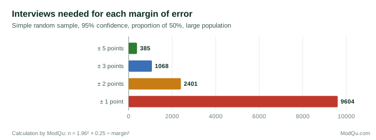
where z is the multiplier for the confidence level (1.96 for 95 per cent), p is the expected proportion and e is the margin of error expressed as a proportion. For p = 0.5 and e = 0.03, this gives 1.96² × 0.25 ÷ 0.0009 ≈ 1,068 completed interviews.
Figure 1 shows how the margin of error falls as the sample grows. The curve flattens quickly: going from 100 to 400 interviews cuts the margin from about ±10 to ±5 points, but going from 1,000 to 3,000 cuts it only from about ±3.1 to ±1.8 points.
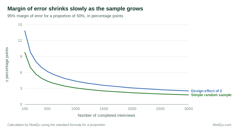
Figure 2 turns the calculation around and shows the number of interviews needed for common margins of error. Each step towards greater precision costs much more than the previous one.
For a mean, the formula is similar, with the population variance in place of p × (1 − p) and the margin expressed in the units of the variable. Interval methods for proportions that are close to 0 or 1 perform better than the simple formula, which can be misleading in those cases (Wilson, 1927; Agresti & Coull, 1998).
Adjusting for the sample design
The basic formula assumes a simple random sample. Most real surveys use stratification, clustering and weighting, which change precision. The design effect is the ratio of the variance under the actual design to the variance under simple random sampling (Kish, 1965). Clustering and unequal weights usually increase it above 1; proportionate stratification can reduce it slightly below 1.
To allow for the design, the simple random sample size is multiplied by the expected design effect. A design effect of 2 doubles the required sample, as the upper line in Figure 1 shows. Kish (1995) provided practical methods for estimating design effects from previous surveys, including the effect of variable weights, which can be approximated as 1 plus the squared coefficient of variation of the weights. Design effects can be large in area-based household surveys and in samples heavily weighted to correct for low response from some groups (Valliant et al., 2018).
Planning for subgroups
Precision for the total sample is often not the binding constraint. If results are needed separately for five regions, each region needs enough interviews on its own. With 1,068 interviews in total, a region containing 10 per cent of the population would have about 107 interviews and a margin of error near ±9.5 points, which may be too imprecise to report.
There are two responses. One is to increase the total sample. The other is to allocate the sample disproportionately, giving small groups more interviews than their population share and then weighting them back. This improves subgroup precision at the cost of some precision for the total, because unequal weights raise the design effect (Kish, 1965; Neyman, 1934).
Small populations
When the population is small, the finite population correction matters. The adjusted sample size is n ÷ (1 + (n − 1) ÷ N), where n is the size from the basic formula and N is the population size. For an organisation with 400 employees that wants a margin of ±3 points, the basic formula gives 1,068, which is more than the whole workforce. After correction, the requirement falls to about 291 completed responses (illustrative calculation).
This calculation exposes a common issue in employee and member surveys. To reach high precision in a small population, a large share of the population must respond. With 400 employees and a 50 per cent response rate, only about 200 responses would be received, giving a margin of about ±4.9 points. In such cases it is usually better to invite everyone and work to maximise response than to sample, and to remember that nonresponse, not sampling, is then the main source of uncertainty.
Averages and rare characteristics
For averages, the calculation needs an estimate of the standard deviation. Suppose a company wants to estimate average monthly spending per customer to within ±5 dollars, and a previous survey found a standard deviation of 60 dollars. The required sample is 1.96² × 60² ÷ 5² ≈ 553 completes (illustrative calculation). If the standard deviation is uncertain, it is safer to plan with a larger value, because an underestimate leads to a sample that is too small.
Rare characteristics pose a different problem. The margin of error for a proportion of 5 per cent is smaller in absolute terms than for 50 per cent, but larger relative to the estimate. With 1,000 interviews, a 5 per cent estimate has a margin of about ±1.4 points, which is more than a quarter of the estimate itself. When the aim is to describe the people who have a rare characteristic, the relevant sample is the number of such people, not the total, and screening a large sample or using special designs may be needed (Kish, 1965).
Sample size for comparisons
When the aim is to compare two groups or two time points, the calculation is based on power: the probability of detecting a real difference of a given size. The researcher specifies the smallest difference that would matter, the significance level (usually 5 per cent) and the desired power (often 80 per cent). Power analysis software such as G*Power performs these calculations for many common tests (Faul et al., 2007).
For example, to detect a change in a proportion from 50 to 55 per cent between two independent samples with 80 per cent power and a 5 per cent significance level, each sample needs roughly 1,560 respondents. Detecting a change from 50 to 60 per cent needs only about 390 per sample (illustrative calculation). The size of the difference that matters therefore has a large effect on cost.
Cohen (1988, 1992) proposed conventional "small", "medium" and "large" effect sizes for use when no other information is available. These conventions are widely used, but critics argue that sample size should be justified by the effect that matters in the specific context, not by generic benchmarks (Lenth, 2001; Lakens, 2022). Underpowered studies are common and can produce exaggerated or even wrongly signed estimates when they do find significant results (Button et al., 2013; Gelman & Carlin, 2014).
A related approach, called accuracy in parameter estimation, plans the sample so that confidence intervals for the key quantities, such as regression coefficients, will be narrow enough to be informative, rather than only large enough for a significance test (Kelley & Maxwell, 2003; Maxwell et al., 2008; Cumming, 2014).
Repeated surveys and panels
Many business surveys are repeated to track change. When independent samples are drawn each time, the variance of the difference between two estimates is the sum of their variances, so detecting change requires larger samples than estimating a single level. When the same people are interviewed each time, as in a panel, their answers are correlated across waves, and the variance of the change is reduced. With a correlation of 0.5 between waves, a panel needs about half the sample of independent samples to detect the same change (Kish, 1965). Panels bring their own problems, such as attrition and conditioning, but where tracking change is the main purpose, the gain in precision can be large.
From completed interviews to issued sample
All the calculations above give the number of completed interviews. The number of people who must be contacted is larger, because some will be ineligible, some cannot be reached and some decline. If a survey needs 1,000 completes, expects 90 per cent of sampled cases to be eligible and expects a response rate of 25 per cent among eligible cases, it must issue about 1,000 ÷ (0.9 × 0.25) ≈ 4,450 cases. Response rates should be calculated using standard definitions so that planning is based on comparable figures (American Association for Public Opinion Research [AAPOR], 2023).
A larger issued sample compensates for low response in terms of numbers, but not in terms of nonresponse bias. A survey with 1,000 completes from a 5 per cent response rate has the same sampling error as one with 1,000 completes from a 60 per cent response rate, but the risk that respondents differ from nonrespondents may be very different (Groves & Peytcheva, 2008).
Budget and the trade-offs
Budget is often the real constraint. The researcher then works backwards: given the money available and the cost per completed interview, how many interviews can be afforded, and what precision does that give? If the answer is not good enough, something must change: the required precision, the number of subgroups, the mode of data collection or the budget itself. For example, with a budget of 30,000 dollars and a cost of 25 dollars per completed online interview, 1,200 completes are affordable, giving a margin of about ±2.8 points. If the same study used telephone interviews at 60 dollars each, only 500 completes would be affordable, with a margin of about ±4.4 points (illustrative figures). The cheaper mode buys precision, but it may bring other errors, such as weaker coverage or different measurement, so the choice cannot rest on sample size alone. Writing these trade-offs down before fieldwork helps sponsors see what they are buying.
Groves (1989) argued that sample size should be considered together with all other sources of error and cost. Money spent on a larger sample is money not spent on reducing nonresponse, improving the questionnaire or checking the frame. Beyond a certain point, extra interviews reduce sampling error by very little, while other errors remain unchanged. In very large samples drawn from biased sources, the bias dominates completely, and adding more cases only makes the estimate more precisely wrong (Meng, 2018).
Rules of thumb and their limits
Published tables, such as the widely cited table by Krejcie and Morgan (1970), give sample sizes for different population sizes at a fixed margin of error and confidence level. They are useful as a quick check but share the assumptions of the basic formula: simple random sampling, a proportion near 50 per cent and no subgroup analysis. Guidance for organisational research makes the same point: tables are a starting point, not a substitute for a calculation based on the study's own needs (Bartlett et al., 2001).
Worked example
A retail chain wants to estimate customer satisfaction nationally with a margin of ±3 points and to report results for four regions with a margin of no more than ±6 points. It expects a design effect of 1.3 from weighting and a response rate of 20 per cent among valid email addresses, of which 95 per cent are expected to be valid (illustrative example).
- National requirement: 1,068 × 1.3 ≈ 1,390 completes.
- Regional requirement: for ±6 points, about 267 completes per region before the design effect, or about 350 after it; four regions need about 1,400 completes.
- The two requirements are similar, so the chain plans for about 1,400 completes, allocating at least 350 to each region.
- Issued sample: 1,400 ÷ (0.95 × 0.20) ≈ 7,370 invitations.
If the budget allows only 1,000 completes, the chain must accept wider margins, about ±3.5 points nationally and ±7 points for regions with 250 completes each, or drop regional reporting for the smallest regions.
Common mistakes
- Choosing a sample size without stating the precision or power it is meant to achieve.
- Calculating precision for the total sample when decisions depend on subgroups.
- Ignoring the design effect of clustering or weighting.
- Confusing completed interviews with issued sample.
- Assuming that a larger sample protects against bias from low response or poor coverage.
- Reporting margins of error for non-probability samples as if they were random samples.
- Using generic effect sizes instead of the smallest difference that would change a decision (Lakens, 2022).
Conclusion
Sample size is not a number to be chosen by habit. It follows from the precision or power the study needs, the confidence level, the variability of the population, the sample design, the subgroups of interest and the expected response. Because precision improves only with the square root of the sample, each gain costs more than the last, and budget forces trade-offs. A good sample size calculation makes those trade-offs explicit and balances sampling error against the other errors that a larger sample cannot fix (Cochran, 1977; Groves, 1989).
References
Agresti, A., & Coull, B. A. (1998). Approximate is better than "exact" for interval estimation of binomial proportions. The American Statistician, 52(2), 119–126. https://doi.org/10.1080/00031305.1998.10480550
American Association for Public Opinion Research. (2023). Standard definitions: Final dispositions of case codes and outcome rates for surveys (10th ed.). AAPOR. https://aapor.org/standards-and-ethics/standard-definitions/
Bartlett, J. E., II, Kotrlik, J. W., & Higgins, C. C. (2001). Organizational research: Determining appropriate sample size in survey research. Information Technology, Learning, and Performance Journal, 19(1), 43–50.
Button, K. S., Ioannidis, J. P. A., Mokrysz, C., Nosek, B. A., Flint, J., Robinson, E. S. J., & Munafò, M. R. (2013). Power failure: Why small sample size undermines the reliability of neuroscience. Nature Reviews Neuroscience, 14(5), 365–376. https://doi.org/10.1038/nrn3475
Cochran, W. G. (1977). Sampling techniques (3rd ed.). Wiley.
Cohen, J. (1988). Statistical power analysis for the behavioral sciences (2nd ed.). Lawrence Erlbaum Associates. https://doi.org/10.4324/9780203771587
Cohen, J. (1992). A power primer. Psychological Bulletin, 112(1), 155–159. https://doi.org/10.1037/0033-2909.112.1.155
Cumming, G. (2014). The new statistics: Why and how. Psychological Science, 25(1), 7–29. https://doi.org/10.1177/0956797613504966
Faul, F., Erdfelder, E., Lang, A.-G., & Buchner, A. (2007). GPower 3: A flexible statistical power analysis program for the social, behavioral, and biomedical sciences. Behavior Research Methods, 39*(2), 175–191. https://doi.org/10.3758/BF03193146
Gelman, A., & Carlin, J. (2014). Beyond power calculations: Assessing Type S (sign) and Type M (magnitude) errors. Perspectives on Psychological Science, 9(6), 641–651. https://doi.org/10.1177/1745691614551642
Groves, R. M., & Peytcheva, E. (2008). The impact of nonresponse rates on nonresponse bias: A meta-analysis. Public Opinion Quarterly, 72(2), 167–189. https://doi.org/10.1093/poq/nfn011
Groves, R. M. (1989). Survey errors and survey costs. Wiley. https://doi.org/10.1002/0471725277
Kelley, K., & Maxwell, S. E. (2003). Sample size for multiple regression: Obtaining regression coefficients that are accurate, not simply significant. Psychological Methods, 8(3), 305–321. https://doi.org/10.1037/1082-989X.8.3.305
Kish, L. (1965). Survey sampling. Wiley.
Kish, L. (1995). Methods for design effects. Journal of Official Statistics, 11(1), 55–77.
Krejcie, R. V., & Morgan, D. W. (1970). Determining sample size for research activities. Educational and Psychological Measurement, 30(3), 607–610. https://doi.org/10.1177/001316447003000308
Lakens, D. (2022). Sample size justification. Collabra: Psychology, 8(1), Article 33267. https://doi.org/10.1525/collabra.33267
Lenth, R. V. (2001). Some practical guidelines for effective sample size determination. The American Statistician, 55(3), 187–193. https://doi.org/10.1198/000313001317098149
Lohr, S. L. (2022). Sampling: Design and analysis (3rd ed.). CRC Press. https://doi.org/10.1201/9780429298899
Maxwell, S. E., Kelley, K., & Rausch, J. R. (2008). Sample size planning for statistical power and accuracy in parameter estimation. Annual Review of Psychology, 59, 537–563. https://doi.org/10.1146/annurev.psych.59.103006.093735
Meng, X.-L. (2018). Statistical paradises and paradoxes in big data (I): Law of large populations, big data paradox, and the 2016 US presidential election. The Annals of Applied Statistics, 12(2), 685–726. https://doi.org/10.1214/18-AOAS1161SF
Neyman, J. (1934). On the two different aspects of the representative method: The method of stratified sampling and the method of purposive selection. Journal of the Royal Statistical Society, 97(4), 558–625. https://doi.org/10.2307/2342192
Valliant, R., Dever, J. A., & Kreuter, F. (2018). Practical tools for designing and weighting survey samples (2nd ed.). Springer. https://doi.org/10.1007/978-3-319-93632-1
Wilson, E. B. (1927). Probable inference, the law of succession, and statistical inference. Journal of the American Statistical Association, 22(158), 209–212. https://doi.org/10.1080/01621459.1927.10502953