
Statistics · Tests and models
Spatial Statistics and Geographic Information Systems in Knowledge Generation
How spatial statistics and geographic information systems turn location into evidence, how to measure and test geographic clustering, and which traps to avoid when mapping survey and business data.
Almost every business record has a location attached: a customer's postal code, a store's address, a respondent's region. Spatial statistics is the branch of statistics that treats that location as information rather than as a label. Geographic information systems (GIS) store, link and display located data; spatial statistics asks whether the patterns on the map are real, how strong they are and what might explain them. Goodchild (1992) argued that the two belong together as a geographic information science, in which the map is a starting point for analysis rather than its end.
Why location changes the analysis
Tobler (1970) summarised the core idea in what is now called the first law of geography: "everything is related to everything else, but near things are more related than distant things." Neighbouring areas share climate, income levels, media markets and word of mouth, so their survey results tend to resemble each other. This spatial autocorrelation has two consequences. It is a source of knowledge, because clusters point to local causes worth investigating. It is also a statistical problem, because most standard tests assume independent observations, and similar neighbours carry less independent information than their number suggests.
Measuring clustering: Moran's I
The classic summary of spatial autocorrelation is Moran's I (Moran, 1950). It works like a correlation coefficient between each area's value and the values of its neighbours:
I = (n ÷ W) × Σi Σj wij(xi − x̄)(xj − x̄) ÷ Σi(xi − x̄)2
Here n is the number of areas, wij is 1 if areas i and j are neighbours and 0 otherwise, and W is the sum of all the weights. Values near +1 indicate that similar values sit together, values near 0 indicate no spatial pattern (the exact expectation is −1 ÷ (n − 1)), and negative values indicate a checkerboard of dissimilar neighbours. Because the theoretical distribution of I depends on the map, significance is usually judged with a permutation test: the values are shuffled across the areas many times, and the observed I is compared with the shuffled ones.
A worked example
Consider a hypothetical brand-awareness survey reported for 64 areas on a regular grid. In Figure 1, panel A shows high awareness concentrated in the north-west and low awareness in the south-east, with Moran's I of 0.82. Panel B contains exactly the same 64 values, shuffled at random. Both maps have the same mean (51.3%), the same spread and the same histogram, yet panel B has Moran's I of −0.01, and none of 999 shuffles of panel A's values produced an I as large as the observed one.
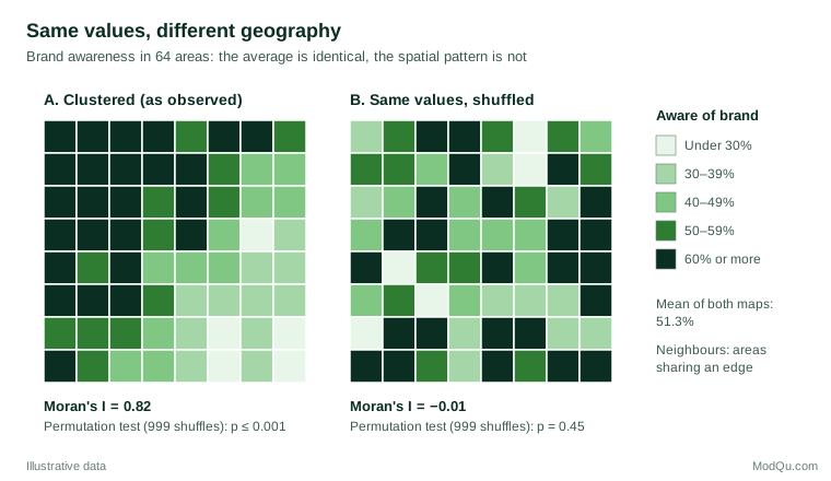
A non-spatial summary cannot tell these two situations apart. For a marketing team, the difference matters: panel A suggests a regional cause, such as distribution gaps or a local competitor, while panel B suggests that awareness varies for reasons unrelated to place.
From global patterns to local knowledge
A single global statistic says whether clustering exists, not where it is. Local indicators of spatial association break Moran's I into a contribution for each area, flagging hot spots, cold spots and outliers such as a low-awareness area surrounded by high ones (Anselin, 1995). The Getis–Ord statistics serve a similar purpose by testing whether high or low values concentrate within a chosen distance of each location (Getis & Ord, 1992).
Other tools model space directly. Kriging, developed in geostatistics, predicts values at unsampled locations from a model of how similarity decays with distance (Matheron, 1963). Geographically weighted regression lets regression coefficients vary across the map, showing, for example, that price sensitivity is stronger in some regions than others (Brunsdon et al., 1996).
Practical guidance and common mistakes
- Choose and report the neighbour definition. Shared borders, distance bands and nearest neighbours can give different answers. Test whether conclusions survive a reasonable alternative.
- Beware the modifiable areal unit problem. Results can change when the same data are aggregated to different boundaries or scales; Fotheringham and Wong (1991) showed that regression results on census data shifted markedly with the zoning system.
- Avoid the ecological fallacy. A correlation between area averages need not hold for individuals; Robinson (1950) showed that area-level correlations can differ greatly from individual-level ones.
- Watch small-sample areas. Areas with few respondents produce extreme percentages by chance, which can look like hot spots. Pool areas, use smoothing or report intervals.
- Adjust inference for autocorrelation. Treating clustered observations as independent understates standard errors; spatial regression models or clustered standard errors are safer.
Key takeaways
Location is a source of knowledge, not just a mailing detail. Spatial statistics measures whether geographic patterns are stronger than chance, locates where they occur and models how relationships vary across space. Used with careful neighbour definitions, sensible area sizes and awareness of aggregation effects, GIS and spatial methods turn a coloured map into evidence that can support decisions.
References
Anselin, L. (1995). Local indicators of spatial association—LISA. Geographical Analysis, 27(2), 93–115. https://doi.org/10.1111/j.1538-4632.1995.tb00338.x
Brunsdon, C., Fotheringham, A. S., & Charlton, M. E. (1996). Geographically weighted regression: A method for exploring spatial nonstationarity. Geographical Analysis, 28(4), 281–298. https://doi.org/10.1111/j.1538-4632.1996.tb00936.x
Fotheringham, A. S., & Wong, D. W. S. (1991). The modifiable areal unit problem in multivariate statistical analysis. Environment and Planning A: Economy and Space, 23(7), 1025–1044. https://doi.org/10.1068/a231025
Getis, A., & Ord, J. K. (1992). The analysis of spatial association by use of distance statistics. Geographical Analysis, 24(3), 189–206. https://doi.org/10.1111/j.1538-4632.1992.tb00261.x
Goodchild, M. F. (1992). Geographical information science. International Journal of Geographical Information Systems, 6(1), 31–45. https://doi.org/10.1080/02693799208901893
Matheron, G. (1963). Principles of geostatistics. Economic Geology, 58(8), 1246–1266. https://doi.org/10.2113/gsecongeo.58.8.1246
Moran, P. A. P. (1950). Notes on continuous stochastic phenomena. Biometrika, 37(1–2), 17–23. https://doi.org/10.1093/biomet/37.1-2.17
Robinson, W. S. (1950). Ecological correlations and the behavior of individuals. American Sociological Review, 15(3), 351–357. https://doi.org/10.2307/2087176
Tobler, W. R. (1970). A computer movie simulating urban growth in the Detroit region. Economic Geography, 46(Suppl. 1), 234–240. https://doi.org/10.2307/143141