
Statistics · Data science and machine learning
Overfitting and the Bias-Variance Trade-off
Why models that fit their data too closely predict badly, how prediction error splits into bias, variance and noise, and the practical tools that keep business models at the right level of complexity.
Every predictive model is a compromise. A model that is too simple misses real patterns in the data; a model that is too flexible learns patterns that are not there. The second failure, overfitting, is the more dangerous of the two because it hides behind excellent results on the data used to build the model. The bias-variance trade-off explains why it happens and points to the remedies (Geman et al., 1992; Hastie et al., 2009).
What overfitting looks like
Imagine fitting a model of purchase intention to 300 survey respondents using 60 candidate predictors, including dozens of interaction terms. With enough flexibility the model can trace almost every respondent's answer, and its R² on the sample may look impressive. But much of what it has learned is noise: the particular quirks of these 300 people that will not recur in the next sample. When the model is applied to new customers, its predictions are worse than those of a far simpler model.
Hawkins (2004) defines overfitting as using a model or procedure that is more complex than necessary, so that it fits the sample but generalises poorly. Babyak (2004) shows how common it is in regression-type models in the behavioural sciences, where many predictors, small samples and data-driven variable selection combine to produce findings that fail to replicate.
The bias-variance decomposition
To see why, consider the expected error of a model's prediction at a new point x, averaged over all the training samples we might have drawn. For squared error it splits into three parts (Geman et al., 1992):
E[(y − f̂(x))2] = Bias[f̂(x)]2 + Var[f̂(x)] + σ2
- Bias is the systematic gap between the average prediction and the truth. Simple models, such as a straight line fitted to a curved relationship, have high bias: no amount of data will fix the wrong shape.
- Variance is how much the fitted model would change if we drew a different sample. Flexible models have high variance because they bend to fit whichever observations they happen to receive.
- Irreducible noise, σ², is the variation in the outcome that no model can predict from the available inputs, such as an individual's mood on the day of the survey.
As complexity increases, bias usually falls and variance rises. Expected test error is their sum plus the noise, so it typically falls at first and then rises again. The best model sits near the bottom of that U, not at the point of best fit to the training data.
A worked simulation
Figure 1 shows a hypothetical example. A curved relationship was simulated, 25 observations were drawn with noise variance 0.12, and polynomial models of degree 1 to 14 were fitted. The process was repeated 3,000 times so that bias and variance could be measured directly.
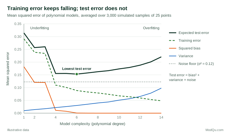
The straight line (degree 1) underfits: its squared bias is 0.18 and its expected test error 0.31. By degree 6 the bias has all but vanished and test error reaches its minimum of 0.15. Beyond that point every extra term adds variance without removing any bias, and by degree 14 the test error has risen to 0.22. Meanwhile, the training error keeps falling, to 0.05 at degree 14, well below the irreducible noise of 0.12. A training error below the noise level is a clear sign that the model is fitting noise.
How to detect overfitting
The decisive check is performance on data the model has not seen: a held-out test set, or cross-validation, in which the data are split into folds and each fold is predicted by a model trained on the rest (Hastie et al., 2009). A large gap between training and validation performance signals high variance; poor performance on both signals high bias. Other warning signs include coefficients that change sharply when a few cases are dropped, and implausibly large effects.
How to control complexity
Use fewer, better predictors
The simplest remedy is to match the number of parameters to the information in the data. For binary outcomes, a simulation study by Peduzzi et al. (1996) found that logistic regression estimates became unreliable with fewer than about 10 events per predictor variable. Harrell (2015) recommends deciding on candidate predictors using subject knowledge before looking at the outcome, and combining or dropping variables rather than letting automated stepwise selection choose them.
Regularise
Regularisation deliberately adds a little bias in exchange for a large reduction in variance. Ridge regression shrinks all coefficients towards zero by penalising their squared size (Hoerl & Kennard, 1970). The lasso penalises their absolute size, which shrinks some coefficients exactly to zero and so performs variable selection at the same time (Tibshirani, 1996). The strength of the penalty is a tuning parameter, normally chosen by cross-validation (James et al., 2021).
Penalise complexity when comparing models
Information criteria trade fit against the number of parameters. The Akaike information criterion (AIC) aims at good predictive accuracy (Akaike, 1974), while the Bayesian information criterion (BIC) applies a stiffer penalty that grows with sample size and tends to select smaller models (Schwarz, 1978).
Average many models
Bagging fits the same flexible model to many bootstrap samples and averages the predictions. Because the individual models' errors partly cancel, the average has much lower variance than any single model (Breiman, 1996). Random forests and many other ensemble methods build on the same idea.
Collect more data
Variance shrinks as the sample grows, so a larger sample supports a more complex model. Domingos (2012) notes that, in practice, a simple method with more data often beats a clever method with less. More data does not help with bias, however: if the model's form is wrong, its error will not fall below the bias however large the sample.
Beyond the classic U-curve
Very large modern models, such as deep neural networks with more parameters than observations, sometimes predict well despite fitting their training data perfectly. Belkin et al. (2019) describe a "double descent" pattern in which test error rises as a model approaches the point where it can just interpolate the data, then falls again as the model becomes even larger. This does not repeal the trade-off; it shows that complexity is not simply the number of parameters. For the moderate-sized data sets typical of survey and business research, the classic U-curve remains the right guide.
Practical guidance for survey and business data
- Count the information, not the rows. For a rare outcome such as a 3% cancellation rate, a sample of 2,000 contains only about 60 events, which supports only a handful of predictors.
- Be wary of many derived variables. Interactions, dummy variables for every brand and region, and repeated recoding all add parameters, even if the analyst thinks of them as one question.
- Validate on later data. Customer behaviour drifts. A model validated on the same survey wave can still fail on the next one.
- Report out-of-sample performance. Present cross-validated or test-set accuracy to stakeholders, not the training R².
Common mistakes
- Choosing among hundreds of candidate models and reporting the winner's performance as if it had been the only model tried.
- Selecting predictors on the full data set before cross-validation, which lets the test folds influence the model.
- Assuming that a more complex model is more accurate because it fits the sample better.
- Treating underfitting as safe. A model with high bias gives consistently wrong answers, which can be just as costly.
Key takeaways
Prediction error has three sources: bias from a model that is too rigid, variance from a model that is too flexible, and noise that no model can remove. Training error measures only how well the model memorises its sample, so judge models on new data. Keep complexity in proportion to the information available, use regularisation, information criteria or averaging to tame variance, and accept a small amount of bias when it buys a large gain in stability.
References
Akaike, H. (1974). A new look at the statistical model identification. IEEE Transactions on Automatic Control, 19(6), 716–723. https://doi.org/10.1109/TAC.1974.1100705
Babyak, M. A. (2004). What you see may not be what you get: A brief, nontechnical introduction to overfitting in regression-type models. Psychosomatic Medicine, 66(3), 411–421. https://doi.org/10.1097/01.psy.0000127692.23278.a9
Belkin, M., Hsu, D., Ma, S., & Mandal, S. (2019). Reconciling modern machine-learning practice and the classical bias–variance trade-off. Proceedings of the National Academy of Sciences, 116(32), 15849–15854. https://doi.org/10.1073/pnas.1903070116
Breiman, L. (1996). Bagging predictors. Machine Learning, 24(2), 123–140. https://doi.org/10.1007/BF00058655
Domingos, P. (2012). A few useful things to know about machine learning. Communications of the ACM, 55(10), 78–87. https://doi.org/10.1145/2347736.2347755
Geman, S., Bienenstock, E., & Doursat, R. (1992). Neural networks and the bias/variance dilemma. Neural Computation, 4(1), 1–58. https://doi.org/10.1162/neco.1992.4.1.1
Harrell, F. E., Jr. (2015). Regression modeling strategies: With applications to linear models, logistic and ordinal regression, and survival analysis (2nd ed.). Springer. https://doi.org/10.1007/978-3-319-19425-7
Hastie, T., Tibshirani, R., & Friedman, J. (2009). The elements of statistical learning: Data mining, inference, and prediction (2nd ed.). Springer. https://doi.org/10.1007/978-0-387-84858-7
Hawkins, D. M. (2004). The problem of overfitting. Journal of Chemical Information and Computer Sciences, 44(1), 1–12. https://doi.org/10.1021/ci0342472
Hoerl, A. E., & Kennard, R. W. (1970). Ridge regression: Biased estimation for nonorthogonal problems. Technometrics, 12(1), 55–67. https://doi.org/10.1080/00401706.1970.10488634
James, G., Witten, D., Hastie, T., & Tibshirani, R. (2021). An introduction to statistical learning: With applications in R (2nd ed.). Springer. https://doi.org/10.1007/978-1-0716-1418-1
Peduzzi, P., Concato, J., Kemper, E., Holford, T. R., & Feinstein, A. R. (1996). A simulation study of the number of events per variable in logistic regression analysis. Journal of Clinical Epidemiology, 49(12), 1373–1379. https://doi.org/10.1016/S0895-4356(96)00236-3
Schwarz, G. (1978). Estimating the dimension of a model. The Annals of Statistics, 6(2), 461–464. https://doi.org/10.1214/aos/1176344136
Tibshirani, R. (1996). Regression shrinkage and selection via the lasso. Journal of the Royal Statistical Society Series B: Statistical Methodology, 58(1), 267–288. https://doi.org/10.1111/j.2517-6161.1996.tb02080.x