
Statistics · Data science and machine learning
Statistics and Machine Learning: Differences and Overlaps
How statistics and machine learning differ in goals, culture and validation, where their methods now overlap, and how business and survey analysts can choose the right approach for each question.
Statistics and machine learning both learn from data, and many of their methods are identical. A logistic regression is taught in introductory statistics courses and in machine learning courses alike. Yet the two fields grew from different communities, ask different questions by default and judge success in different ways. For organisations that buy, analyse and act on data, understanding those differences matters more than choosing a side. It explains why a model that predicts churn very well may say little about why customers leave, and why a carefully estimated effect from a survey may predict individual behaviour poorly.
This article sets out the main differences, the large and growing overlap, and practical guidance for choosing an approach in market research and business analytics.
Two origins
Statistics developed from the late nineteenth century as the science of drawing conclusions about populations from samples, with explicit statements of uncertainty. Its central tools, such as sampling theory, hypothesis testing, confidence intervals and experimental design, were built for settings where data were scarce and expensive to collect. Tukey (1962) argued early that data analysis was a broader scientific activity than mathematical statistics, one that should be judged by its usefulness rather than its mathematical elegance.
Machine learning grew from computer science and pattern recognition research, where the aim was to build systems that improve at a task with experience. Its natural measure of success is performance on new cases: how accurately a system recognises an image, ranks a search result or predicts a purchase. Its growth was driven by large data sets and cheap computing, culminating in deep learning methods that learn layered representations directly from raw inputs such as images, text and sound (LeCun et al., 2015).
Breiman (2001a) famously described these as "two cultures". The data-modelling culture assumes that a stochastic model generated the data, estimates that model's parameters and draws conclusions from them. The algorithmic-modelling culture treats the mechanism inside the "black box" as unknown and judges methods by predictive accuracy alone. Breiman, a statistician who had worked as a consultant, argued that statistics had relied too heavily on the first culture and risked irrelevance. Donoho (2017) later argued that much of what is now called data science fulfils Tukey's earlier programme, with prediction and computing at its centre.
The core difference: explaining versus predicting
The clearest way to see the difference is through the question being asked. Shmueli (2010) distinguishes explanatory modelling, which tests or estimates causal or theoretical relationships, from predictive modelling, which aims to forecast new or future observations as accurately as possible. The two goals lead to different choices at every stage: which variables to include, how to handle collinearity, how complex the model should be and how to evaluate it. A model that is best for explanation is often not the best for prediction, and vice versa.
Mullainathan and Spiess (2017) put the same point in notation. Much of traditional statistics and econometrics is concerned with β̂ problems: estimating a parameter, such as the effect of price on demand, with a known degree of uncertainty. Machine learning excels at ŷ problems: producing good predictions of an outcome. Machine learning algorithms can produce excellent ŷ while their internal parameters remain unstable and hard to interpret. If two survey variables are highly correlated, a prediction algorithm may use either one, and which one it picks can change from sample to sample without affecting accuracy.
Efron (2020) adds a third goal, attribution: assigning importance or significance to individual predictors. Traditional regression was designed to do prediction, estimation and attribution at once. Modern prediction algorithms such as random forests and deep networks are excellent at prediction but are not designed for the other two tasks, and their variable-importance measures should not be read as estimates of effects.
A related summary is offered by Bzdok et al. (2018): statistics draws population inferences from a sample, while machine learning finds generalisable predictive patterns. Both are valid aims. Problems arise when an analyst uses a tool built for one aim to answer a question of the other kind.
Different words for the same ideas
Part of the apparent gap between the fields is vocabulary. The same concept often has two names, which can make collaboration between statisticians and data scientists harder than it needs to be (Hastie et al., 2009).
| Statistics | Machine learning |
|---|---|
| Response or dependent variable | Label or target |
| Explanatory variable or covariate | Feature or input |
| Estimating or fitting a model | Training or learning |
| Observation or case | Example or instance |
| Regression and classification | Supervised learning |
| Cluster analysis, latent class analysis | Unsupervised learning |
| Shrinkage or penalised estimation | Regularisation or weight decay |
Translating terms is a small step, but it helps teams see that many disagreements are about goals and assumptions rather than about methods.
How each field validates its models
The two traditions also differ in how they check that a model is good.
Statistics relies largely on theory. If the model's assumptions hold, standard errors, confidence intervals and tests describe the uncertainty in the estimates. Diagnostic checks of residuals and goodness of fit test whether the assumptions are reasonable. Model choice often uses criteria that penalise complexity, and the final model is judged partly by whether its parameters make substantive sense.
Machine learning relies mainly on held-out data. The data are split into training and test sets, or cross-validation is used, in which the model is repeatedly fitted on part of the data and evaluated on the remainder (Stone, 1974). The model that predicts the held-out cases best is preferred, whether or not its structure is interpretable.
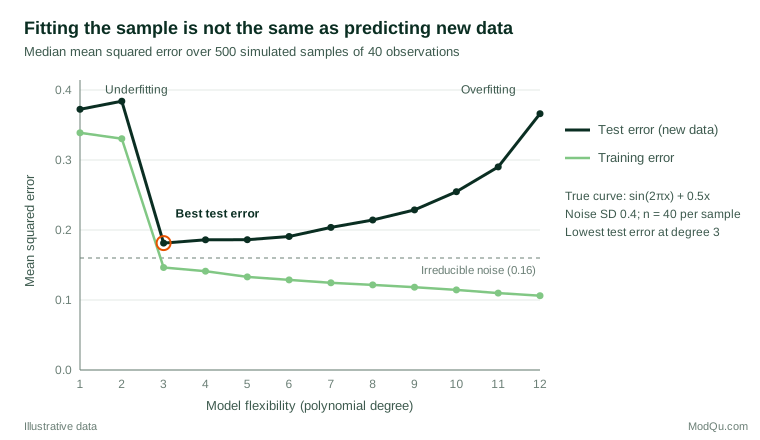
Figure 1 shows why held-out evaluation is essential for prediction. In a simulated example, polynomial models of increasing flexibility were fitted to small samples. Training error falls steadily as flexibility increases, because a more flexible model can always fit the sample more closely. Error on new data falls at first, reaches its lowest value at a moderate level of flexibility, then rises again as the model begins to fit noise. This is the bias–variance trade-off described in standard texts (Hastie et al., 2009; James et al., 2013).
Very large models complicate this picture. Belkin et al. (2019) documented a "double descent" pattern in which test error can fall again once a model has enough parameters to fit the training data exactly. The finding does not remove the need for validation. It shows that the relationship between model size and accuracy must be checked empirically rather than assumed.
Where the fields overlap
The boundary between the fields has largely dissolved at the level of methods (Figure 2). Many tools now regarded as machine learning came from statisticians, and statistical practice has absorbed ideas from computer science.
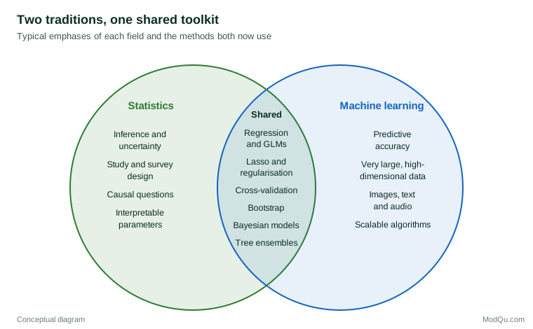
- Regularisation. The lasso shrinks regression coefficients and sets some exactly to zero, trading a little bias for a large reduction in variance (Tibshirani, 1996). It is used for prediction and for selecting variables from long lists of survey items.
- Tree ensembles. Random forests average many decision trees grown on bootstrap samples (Breiman, 2001b), and gradient boosting builds trees one after another to correct the errors of earlier ones (Friedman, 2001). Both were developed by statisticians and are now standard machine learning tools.
- Resampling. Cross-validation (Stone, 1974) and the bootstrap underpin model assessment in both fields.
- Probabilistic models. Bayesian methods, generalised linear models and mixture models are taught in both traditions.
Efron and Hastie (2016) trace how computation reshaped statistical inference itself, so that methods once impossible to compute are now routine. The two fields increasingly share journals, conferences, software and people.
The overlap also runs the other way. Causal inference, a traditional strength of statistics and econometrics, now uses machine learning as a component. Double/debiased machine learning uses flexible algorithms to model the relationships between confounders, treatment and outcome, then combines them in a way that still gives valid confidence intervals for the causal effect (Chernozhukov et al., 2018). Causal forests adapt random forests to estimate how a treatment effect varies across individuals, with valid statistical inference (Wager & Athey, 2018). Athey and Imbens (2019) review these and other machine learning methods that economists and social scientists can use for causal questions.
A worked example: churn prediction versus churn drivers
Consider a hypothetical subscription company with a customer survey of 5,000 respondents linked to records of who cancelled in the following six months. Management asks two questions that sound similar but are not.
Question 1: Which customers are most likely to cancel? This is a ŷ problem. The goal is to rank customers so that a retention team can contact the right ones. A gradient-boosted model using all survey answers, usage data and account history might be the best choice. It should be judged on held-out data, for example by how many actual cancellations fall in the top 10% of predicted risk. Interpretability is useful but secondary.
Question 2: Would improving onboarding reduce cancellations? This is a causal β̂ problem. A high importance score for an onboarding satisfaction item in the boosted model does not answer it. The item may simply be correlated with other drivers, such as customer size or product tier. Answering the question needs an explanatory design: a randomised test of a new onboarding process, or an observational analysis that adjusts carefully for confounders and reports uncertainty. Machine learning can help in that analysis, as in double/debiased methods, but the question and the design come first.
Many analytics failures come from answering Question 2 with tools built for Question 1. The reverse mistake also occurs: a simple, well-specified regression may estimate the onboarding effect well but rank individual customers poorly, because it leaves out complex interactions that a flexible algorithm would capture.
Practical guidance for survey and business data
- State the goal first. Write down whether the task is description, prediction or causal explanation (Shmueli, 2010). The answer determines the method, the validation strategy and how results should be reported.
- Respect the sample. Prediction algorithms assume that new cases come from the same population as the training data. Survey data often come from weighted or non-random samples, and models trained on one customer base or period may not transfer to another. Statistical thinking about populations and sampling remains essential.
- Validate honestly. Keep a test set untouched until the end, and use cross-validation for tuning. For data collected over time, test on later periods rather than random splits, because the future may differ from the past.
- Report uncertainty. A single accuracy figure hides variation. Report intervals for accuracy measures and effect estimates, and show how results change across reasonable modelling choices.
- Prefer simpler models when they perform comparably. Hand (2006) showed that simple classifiers often achieve most of the predictive gain of more complex ones, and that apparent improvements from sophisticated methods can vanish when real-world conditions differ from the test data. A simpler model is easier to explain, audit and maintain.
- Plan for explanation to stakeholders. Decisions that affect customers, such as who receives an offer or a price change, often need to be justified to managers, regulators or the customers themselves. Where a complex model is used, document its inputs, test its behaviour across customer segments and keep a simpler benchmark model for comparison.
- Beware of scale without design. Large volumes of data do not replace a sound design. Google Flu Trends, which estimated influenza activity from search queries, substantially overestimated influenza levels in later seasons. Lazer et al. (2014) attributed this partly to "big data hubris", the assumption that large data sets can substitute for traditional data collection and analysis, and to changes in the search algorithm itself.
Common misconceptions
- "Machine learning is just statistics rebranded." Many methods are shared, but machine learning has made distinctive contributions in algorithms, scale, and learning from unstructured data such as images and text.
- "Statistics is only for small data." Statistical ideas about sampling, bias, uncertainty and causation matter more, not less, when data sets are large but unrepresentative.
- "A model that predicts well must have found the causes." High predictive accuracy is compatible with entirely non-causal relationships.
- "Variable importance equals effect size." Importance scores describe how an algorithm uses inputs, not what would happen if those inputs changed (Efron, 2020).
- "Interpretable models are always less accurate." For many structured business data sets, carefully specified regression models perform close to complex algorithms (Hand, 2006).
Key takeaways
Statistics and machine learning share much of their toolkit but differ in emphasis. Statistics focuses on inference about populations, uncertainty, design and explanation. Machine learning focuses on predictive accuracy on new data, scalable algorithms and complex inputs. The most useful distinction for practitioners is not between fields but between questions: prediction problems call for flexible models judged on held-out data, while causal and explanatory problems call for careful design, interpretable estimates and honest statements of uncertainty. The strongest modern methods, such as double/debiased machine learning and causal forests, combine both traditions. Business and survey analysts gain most by choosing tools to suit the question rather than the label.
References
Athey, S., & Imbens, G. W. (2019). Machine learning methods that economists should know about. Annual Review of Economics, 11, 685–725. https://doi.org/10.1146/annurev-economics-080217-053433
Belkin, M., Hsu, D., Ma, S., & Mandal, S. (2019). Reconciling modern machine-learning practice and the classical bias–variance trade-off. Proceedings of the National Academy of Sciences, 116(32), 15849–15854. https://doi.org/10.1073/pnas.1903070116
Breiman, L. (2001a). Statistical modeling: The two cultures (with comments and a rejoinder by the author). Statistical Science, 16(3), 199–231. https://doi.org/10.1214/ss/1009213726
Breiman, L. (2001b). Random forests. Machine Learning, 45(1), 5–32. https://doi.org/10.1023/A:1010933404324
Bzdok, D., Altman, N., & Krzywinski, M. (2018). Statistics versus machine learning. Nature Methods, 15(4), 233–234. https://doi.org/10.1038/nmeth.4642
Chernozhukov, V., Chetverikov, D., Demirer, M., Duflo, E., Hansen, C., Newey, W., & Robins, J. (2018). Double/debiased machine learning for treatment and structural parameters. The Econometrics Journal, 21(1), C1–C68. https://doi.org/10.1111/ectj.12097
Donoho, D. (2017). 50 years of data science. Journal of Computational and Graphical Statistics, 26(4), 745–766. https://doi.org/10.1080/10618600.2017.1384734
Efron, B. (2020). Prediction, estimation, and attribution. Journal of the American Statistical Association, 115(530), 636–655. https://doi.org/10.1080/01621459.2020.1762613
Efron, B., & Hastie, T. (2016). Computer age statistical inference: Algorithms, evidence, and data science. Cambridge University Press. https://doi.org/10.1017/CBO9781316576533
Friedman, J. H. (2001). Greedy function approximation: A gradient boosting machine. The Annals of Statistics, 29(5), 1189–1232. https://doi.org/10.1214/aos/1013203451
Hand, D. J. (2006). Classifier technology and the illusion of progress. Statistical Science, 21(1), 1–14. https://doi.org/10.1214/088342306000000060
Hastie, T., Tibshirani, R., & Friedman, J. (2009). The elements of statistical learning: Data mining, inference, and prediction (2nd ed.). Springer. https://doi.org/10.1007/978-0-387-84858-7
James, G., Witten, D., Hastie, T., & Tibshirani, R. (2013). An introduction to statistical learning: With applications in R. Springer. https://doi.org/10.1007/978-1-4614-7138-7
Lazer, D., Kennedy, R., King, G., & Vespignani, A. (2014). The parable of Google Flu: Traps in big data analysis. Science, 343(6176), 1203–1205. https://doi.org/10.1126/science.1248506
LeCun, Y., Bengio, Y., & Hinton, G. (2015). Deep learning. Nature, 521(7553), 436–444. https://doi.org/10.1038/nature14539
Mullainathan, S., & Spiess, J. (2017). Machine learning: An applied econometric approach. Journal of Economic Perspectives, 31(2), 87–106. https://doi.org/10.1257/jep.31.2.87
Shmueli, G. (2010). To explain or to predict? Statistical Science, 25(3), 289–310. https://doi.org/10.1214/10-STS330
Stone, M. (1974). Cross-validatory choice and assessment of statistical predictions. Journal of the Royal Statistical Society Series B: Statistical Methodology, 36(2), 111–133. https://doi.org/10.1111/j.2517-6161.1974.tb00994.x
Tibshirani, R. (1996). Regression shrinkage and selection via the lasso. Journal of the Royal Statistical Society Series B: Statistical Methodology, 58(1), 267–288. https://doi.org/10.1111/j.2517-6161.1996.tb02080.x
Tukey, J. W. (1962). The future of data analysis. The Annals of Mathematical Statistics, 33(1), 1–67. https://doi.org/10.1214/aoms/1177704711
Wager, S., & Athey, S. (2018). Estimation and inference of heterogeneous treatment effects using random forests. Journal of the American Statistical Association, 113(523), 1228–1242. https://doi.org/10.1080/01621459.2017.1319839