
Statistics · Causal inference
Confounding Variables and How to Control for Them
What makes a variable a confounder, which variables should and should not be adjusted for, and how stratification, regression, matching and propensity-score weighting control confounding in survey and business data.
A telecoms survey finds that customers who use the company's mobile app are 17 percentage points more likely to say they are satisfied. The product team concludes that the app drives satisfaction and proposes a campaign to push app adoption. Before anyone signs off, a statistician asks a simple question: who uses the app? If long-standing customers are both more likely to have downloaded it and more likely to be satisfied for other reasons, part or all of the 17-point gap reflects tenure, not the app. Tenure would then be a confounder.
Confounding is the most common reason why associations in observational data differ from causal effects. This article explains what a confounder is, how to decide which variables need controlling for, which methods do the controlling and how to judge whether the job has been done well enough to support a decision.
What makes a variable a confounder
In the traditional epidemiological definition, a confounder is a variable that is associated with the exposure, is associated with the outcome independently of the exposure, and is not itself an effect of the exposure (Rothman et al., 2008). In the app example, tenure is associated with app use, affects satisfaction directly and is not caused by using the app.
Modern causal inference gives a sharper definition. Confounding is present when the exposed and unexposed groups would have had different outcomes even if the exposure had no effect; in other words, when they are not exchangeable (Greenland & Morgenstern, 2001). A confounder is a variable that helps to create that difference, typically a common cause of both exposure and outcome. Drawn as a causal diagram, it sits on a "back-door" path: an arrow runs from the confounder into the exposure, and another runs from the confounder to the outcome (Greenland et al., 1999; Pearl, 2009).
The structural definition matters because statistical association alone cannot tell a confounder from other kinds of variable. A variable can be correlated with both exposure and outcome and still be something that must not be adjusted for, as the next section shows.
Confounders, mediators and colliders
Three types of third variable look similar in a correlation table but call for opposite treatment.
- Confounder (common cause). Affects both exposure and outcome. Adjusting for it removes bias.
- Mediator (on the causal path). Is affected by the exposure and in turn affects the outcome. Adjusting for it removes part of the effect being estimated. Schisterman et al. (2009) call this overadjustment bias.
- Collider (common effect). Is affected by both exposure and outcome, or by causes of each. Adjusting for it, or selecting the sample on it, creates a spurious association where none existed (Elwert & Winship, 2014; Hernán et al., 2004).
Figure 1 shows what happens when these rules are broken, using simulated data in which the true answer is known. A software company wants the effect of attending an onboarding webinar on accounts' 12-month spend. Larger accounts are more likely to attend and also spend more: account size is a confounder. Attending the webinar increases product adoption, which raises spend: adoption is a mediator. And accounts that attended or spent more are more likely to answer a follow-up survey: survey response is a collider.
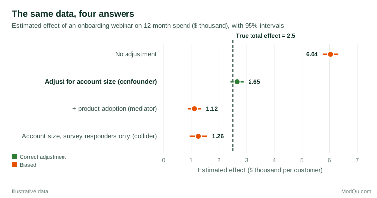
The unadjusted estimate, about $6,000 per account, is more than twice the truth because large accounts both attend and spend. Adjusting for account size brings the estimate to about $2,650, close to the true $2,500. Adding product adoption to the model cuts the estimate to about $1,100, because most of the webinar's effect works through adoption. Restricting the analysis to survey responders also distorts the result, giving about $1,260. Among responders, an account that did not attend the webinar must have had some other reason to respond, such as unusually high spend, so the comparison is tilted against the webinar. Each wrong choice produces a precise-looking estimate with a narrow interval, so the statistical output gives no warning.
Choosing what to control for
Because the right adjustment depends on causal structure, it cannot be chosen by statistical tests, stepwise selection or by entering every available variable. Three practical approaches help.
Draw the diagram. Write down the assumed causal relationships between exposure, outcome and candidate covariates as a directed acyclic graph. The back-door criterion then identifies sufficient adjustment sets (Pearl, 2009). Free software such as DAGitty finds these sets automatically and lists the testable implications of the diagram (Textor et al., 2016).
Use a robust rule when the diagram is uncertain. VanderWeele (2019) proposes a practical criterion: control for every pre-exposure covariate that is a cause of the exposure, the outcome or both; exclude variables known to affect the exposure but not the outcome (instrumental variables); and include good proxies for unmeasured common causes. This rule works even when the full diagram is not known.
Respect time order. As a default, only variables measured before the exposure qualify as confounders. Variables measured afterwards may be mediators or colliders. In surveys that ask about attitudes and behaviour at the same time, this means thinking carefully about what could have changed as a result of the exposure.
For propensity-score models specifically, Brookhart et al. (2006) found in simulations that including variables related to the outcome improved estimates, while including variables related only to the exposure increased variance without reducing bias.
Methods of control
Confounding can be controlled at the design stage, before data are collected, or at the analysis stage.
Design: randomisation, restriction and matching
Randomisation is the only method that controls confounders that are unmeasured or unknown, and it is the subject of a separate article. Restriction limits the study to one level of a confounder, for example only customers in their first year. It removes confounding by that variable completely, at the cost of narrower conclusions. Matching selects comparison units that resemble treated units on key confounders. In a customer study, each new app user might be paired with a non-user of the same tenure band, region and spending level. Matching makes the comparison easy to explain, but it can discard many unmatched units, and the variables used for matching must still be handled correctly in the analysis.
Analysis: stratification and standardisation
The most transparent analytic method is stratification: compare exposed and unexposed units within levels of the confounder, then combine the results. Table 1 applies it to the hypothetical app survey, with tenure in two strata.
| Tenure | App users: n | App users: % satisfied | Non-users: n | Non-users: % satisfied | Difference (points) |
|---|---|---|---|---|---|
| Under 1 year | 200 | 60 | 600 | 54 | 6 |
| 1 year or more | 600 | 82 | 200 | 76 | 6 |
| All customers (crude) | 800 | 76.5 | 800 | 59.5 | 17 |
Table 1. App use and satisfaction by tenure in a hypothetical survey of 1,600 customers.
Within each tenure group, app users are 6 points more satisfied. The crude difference of 17 points is inflated because app users are concentrated among established customers, who are more satisfied anyway. Standardising both groups to the same tenure mix (here 50% in each stratum) gives 71% for users and 65% for non-users, the same 6-point difference. For ratio measures, the Mantel-Haenszel method pools stratum-specific estimates into a single adjusted value (Mantel & Haenszel, 1959).
Stratification is limited by the number of strata. With several confounders, each with several levels, cells quickly become empty. Cochran (1968) showed, however, that even coarse stratification removes most of the bias from a single continuous confounder: five strata remove roughly 90%.
Analysis: regression adjustment
Multiple regression extends stratification to many confounders at once by modelling the outcome as a function of the exposure and the covariates. It is efficient and familiar, but it relies on the model being correctly specified, and it will extrapolate silently if treated and untreated units have little overlap on the covariates. Only the coefficient on the exposure should be interpreted causally; the coefficients on the confounders are not adjusted for their own confounders and should not be read as causal effects (Westreich & Greenland, 2013).
Analysis: propensity scores
The propensity score is the probability that a unit receives the exposure, given its measured covariates. Rosenbaum and Rubin (1983) showed that units with the same propensity score have, on average, the same distribution of those covariates, whatever their exposure. The many covariates can therefore be balanced by balancing a single score. The score is usually estimated with logistic regression and then used in one of four ways (Austin, 2011):
- Matching, which pairs each exposed unit with one or more unexposed units with a similar score (Stuart, 2010);
- Stratification on the score, often into five groups, following Cochran's result;
- Inverse probability weighting, in which each unit is weighted by the inverse of the probability of the exposure it actually received, creating a weighted sample in which exposure is unrelated to the measured covariates (Robins et al., 2000);
- Covariate adjustment using the score in a regression model.
Propensity-score methods separate the design of the comparison from the analysis of outcomes. The analyst can build and check the comparison groups without looking at the outcome, which reduces the temptation to keep adjusting until a preferred answer appears.
Checking balance
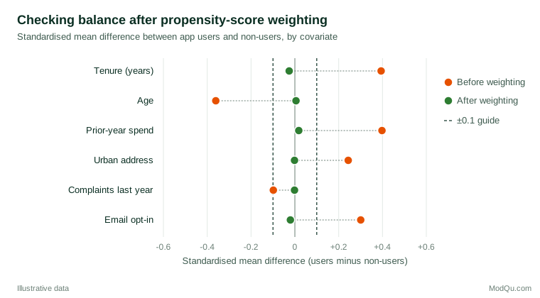
Whichever method is used, the essential diagnostic is whether the adjusted groups are similar on the measured confounders. The standard measure is the standardised mean difference: the difference in means between groups divided by the pooled standard deviation. A common rule of thumb treats absolute values below 0.1 as negligible imbalance (Austin, 2011). Significance tests are a poor guide, because they depend on sample size (Stuart, 2010).
Figure 2 shows a balance check for a hypothetical analysis of app users. Before weighting, users have longer tenure, are younger, spent more last year and are more likely to have opted in to email, with absolute standardised differences between 0.24 and 0.40 on five of the six covariates. After inverse probability weighting on the propensity score, every difference is within 0.03 of zero.
Two cautions apply. Good balance on measured covariates says nothing about unmeasured ones. And when some units have propensity scores close to 0 or 1, the groups barely overlap, weights become extreme and estimates become unstable. Trimming the sample to the region of overlap is often better than forcing a comparison the data cannot support.
Time-varying confounding
In longitudinal data, a confounder can itself be affected by earlier exposure. For example, a customer's engagement score may influence whether they receive a retention offer this month and may also have been raised by last month's offer. Standard regression cannot handle this, because the variable is both a confounder and a mediator. Inverse probability weighting with marginal structural models was developed for exactly this situation (Robins et al., 2000).
When confounders are not measured
Every method above controls only for measured confounders. In business data, important ones are often missing: motivation, household income, competitor offers, a customer's intention to leave. Several approaches address this gap.
Designs that do not rely on measurement. Instrumental variables, difference-in-differences and regression discontinuity designs can remove confounding by unmeasured factors under their own assumptions (Angrist & Pischke, 2009).
Negative controls. A negative control outcome is one that the exposure cannot plausibly affect but that shares the same confounders. If app use appears to "improve" satisfaction with something the app cannot influence, such as the speed of in-store service, residual confounding is likely (Lipsitch et al., 2010).
Sensitivity analysis. Sensitivity analysis asks how strong an unmeasured confounder would have to be to change the conclusion. The idea goes back to the debate over smoking and lung cancer, in which Cornfield et al. (1959) showed that a hidden factor could explain the association away only if it were more strongly associated with smoking than smoking was with lung cancer. Rosenbaum (2002) developed formal bounds for matched studies. The E-value gives the minimum strength of association, on the risk ratio scale, that an unmeasured confounder would need with both exposure and outcome to explain an estimate away (VanderWeele & Ding, 2017). For regression, Cinelli and Hazlett (2020) express the same question in terms of how much variance a confounder would need to explain, and compare it with the strongest measured covariate.
Measurement quality. A confounder measured with error, or grouped into a few broad categories, is only partly controlled. Adjusting for "tenure: under or over five years" leaves residual confounding within each band.
Practical guidance for survey and business data
- Plan confounders into the questionnaire. Decide at the design stage which variables could drive both the exposure and the outcome of interest, and measure them, ideally referring to the period before the exposure.
- Record timing. Ask when customers started using a product or service, not only whether they use it, so that pre-exposure variables can be distinguished from consequences.
- Combine survey and behavioural data. Transaction histories provide pre-exposure measures, such as prior spend, that are hard to collect reliably in a survey.
- Keep weighting purposes separate. Survey weights adjust the sample to the population; propensity weights adjust the comparison groups to each other. When both are needed, they can be combined, but the purposes should be stated.
- Report crude and adjusted estimates. Showing both, with the list of adjustment variables and balance diagnostics, lets readers see how much adjustment mattered.
Common mistakes
- Adjusting for everything available. Some variables are mediators or colliders, and adjusting for them introduces bias.
- Choosing confounders by statistical significance. Whether a variable is a confounder depends on causal structure, not on its p-value in the outcome model.
- Treating adjusted estimates as unconfounded. Adjustment removes bias from measured confounders only. The phrase "after controlling for demographics" does not rule out confounding by attitudes, needs or circumstances.
- Ignoring overlap. If almost all large accounts attend the webinar, the data cannot say what large accounts would have spent without it.
- Interpreting confounder coefficients as effects. Only the exposure coefficient has the causal interpretation the model was built for.
Key takeaways
A confounder is a common cause of exposure and outcome that makes the compared groups non-exchangeable. Identifying confounders is a causal question, best answered with an explicit diagram and with care to exclude mediators and colliders. Stratification, regression, matching and propensity-score weighting all control measured confounders; their success should be judged by balance and overlap diagnostics rather than by model fit. Unmeasured confounding remains the central threat to any observational conclusion, so credible analyses combine careful adjustment with negative controls, sensitivity analysis and, where possible, designs or experiments that do not depend on measuring every confounder.
References
Angrist, J. D., & Pischke, J.-S. (2009). Mostly harmless econometrics: An empiricist's companion. Princeton University Press. https://doi.org/10.1515/9781400829828
Austin, P. C. (2011). An introduction to propensity score methods for reducing the effects of confounding in observational studies. Multivariate Behavioral Research, 46(3), 399–424. https://doi.org/10.1080/00273171.2011.568786
Brookhart, M. A., Schneeweiss, S., Rothman, K. J., Glynn, R. J., Avorn, J., & Stürmer, T. (2006). Variable selection for propensity score models. American Journal of Epidemiology, 163(12), 1149–1156. https://doi.org/10.1093/aje/kwj149
Cinelli, C., & Hazlett, C. (2020). Making sense of sensitivity: Extending omitted variable bias. Journal of the Royal Statistical Society Series B: Statistical Methodology, 82(1), 39–67. https://doi.org/10.1111/rssb.12348
Cochran, W. G. (1968). The effectiveness of adjustment by subclassification in removing bias in observational studies. Biometrics, 24(2), 295–313. https://doi.org/10.2307/2528036
Cornfield, J., Haenszel, W., Hammond, E. C., Lilienfeld, A. M., Shimkin, M. B., & Wynder, E. L. (1959). Smoking and lung cancer: Recent evidence and a discussion of some questions. Journal of the National Cancer Institute, 22(1), 173–203. https://doi.org/10.1093/jnci/22.1.173
Elwert, F., & Winship, C. (2014). Endogenous selection bias: The problem of conditioning on a collider variable. Annual Review of Sociology, 40, 31–53. https://doi.org/10.1146/annurev-soc-071913-043455
Greenland, S., & Morgenstern, H. (2001). Confounding in health research. Annual Review of Public Health, 22, 189–212. https://doi.org/10.1146/annurev.publhealth.22.1.189
Greenland, S., Pearl, J., & Robins, J. M. (1999). Causal diagrams for epidemiologic research. Epidemiology, 10(1), 37–48. https://doi.org/10.1097/00001648-199901000-00008
Hernán, M. A., Hernández-Díaz, S., & Robins, J. M. (2004). A structural approach to selection bias. Epidemiology, 15(5), 615–625. https://doi.org/10.1097/01.ede.0000135174.63482.43
Lipsitch, M., Tchetgen Tchetgen, E., & Cohen, T. (2010). Negative controls: A tool for detecting confounding and bias in observational studies. Epidemiology, 21(3), 383–388. https://doi.org/10.1097/EDE.0b013e3181d61eeb
Mantel, N., & Haenszel, W. (1959). Statistical aspects of the analysis of data from retrospective studies of disease. Journal of the National Cancer Institute, 22(4), 719–748. https://doi.org/10.1093/jnci/22.4.719
Pearl, J. (2009). Causality: Models, reasoning, and inference (2nd ed.). Cambridge University Press. https://doi.org/10.1017/CBO9780511803161
Robins, J. M., Hernán, M. A., & Brumback, B. (2000). Marginal structural models and causal inference in epidemiology. Epidemiology, 11(5), 550–560. https://doi.org/10.1097/00001648-200009000-00011
Rosenbaum, P. R. (2002). Observational studies (2nd ed.). Springer. https://doi.org/10.1007/978-1-4757-3692-2
Rosenbaum, P. R., & Rubin, D. B. (1983). The central role of the propensity score in observational studies for causal effects. Biometrika, 70(1), 41–55. https://doi.org/10.1093/biomet/70.1.41
Rothman, K. J., Greenland, S., & Lash, T. L. (2008). Modern epidemiology (3rd ed.). Lippincott Williams & Wilkins.
Schisterman, E. F., Cole, S. R., & Platt, R. W. (2009). Overadjustment bias and unnecessary adjustment in epidemiologic studies. Epidemiology, 20(4), 488–495. https://doi.org/10.1097/EDE.0b013e3181a819a1
Stuart, E. A. (2010). Matching methods for causal inference: A review and a look forward. Statistical Science, 25(1), 1–21. https://doi.org/10.1214/09-STS313
Textor, J., van der Zander, B., Gilthorpe, M. S., Liśkiewicz, M., & Ellison, G. T. H. (2016). Robust causal inference using directed acyclic graphs: The R package 'dagitty'. International Journal of Epidemiology, 45(6), 1887–1894. https://doi.org/10.1093/ije/dyw341
VanderWeele, T. J. (2019). Principles of confounder selection. European Journal of Epidemiology, 34(3), 211–219. https://doi.org/10.1007/s10654-019-00494-6
VanderWeele, T. J., & Ding, P. (2017). Sensitivity analysis in observational research: Introducing the E-value. Annals of Internal Medicine, 167(4), 268–274. https://doi.org/10.7326/M16-2607
Westreich, D., & Greenland, S. (2013). The Table 2 fallacy: Presenting and interpreting confounder and modifier coefficients. American Journal of Epidemiology, 177(4), 292–298. https://doi.org/10.1093/aje/kws412