
Statistics · Data science and machine learning
Classification Models and Their Evaluation Metrics
A guide to the main classification models and to the metrics used to judge them, from the confusion matrix and accuracy to ROC curves, precision-recall, calibration and cost-based thresholds.
Many of the predictions businesses care about are categories rather than numbers. Will this customer cancel? Is this survey response fraudulent? Which of four segments does this respondent belong to? Models that assign cases to categories are called classification models, or classifiers. Building one is routine; judging it is harder, because a headline figure such as "92% accurate" can hide a model that is useless for the task. This article describes the main families of classifier and then explains, with a worked example, how to evaluate them.
What a classifier produces
Most classifiers do not output a category directly. They output a score for each case, usually an estimated probability that the case belongs to the class of interest, conventionally called the positive class. A category is produced only when the score is compared with a threshold: customers with a predicted churn probability above 0.2, say, are flagged as likely to cancel. This two-step structure matters for evaluation. Some metrics judge the scores themselves, across all possible thresholds; others judge the yes/no decisions at one chosen threshold. Keeping the two apart avoids much confusion.
Common classification models
Logistic regression models the log-odds of the positive class as a linear function of the predictors (Hosmer et al., 2013). It is transparent, produces well-behaved probabilities when its assumptions hold, and remains a strong benchmark for survey data with a modest number of predictors.
Decision trees split the data repeatedly on the predictor values that best separate the classes, producing a set of easy-to-read rules. Single trees are unstable: small changes in the data can produce a very different tree.
Random forests average the votes of hundreds of trees, each grown on a bootstrap sample of the data and using a random subset of predictors at each split (Breiman, 2001). Averaging greatly reduces the instability of single trees.
Gradient boosting builds trees in sequence, each one fitted to correct the errors of the ensemble so far (Friedman, 2001). Boosted trees are often among the most accurate methods for tabular business data, at the price of more tuning.
Support vector machines find the boundary that separates the classes with the widest possible margin, using kernel functions to allow curved boundaries (Cortes & Vapnik, 1995). Their raw outputs are distances from the boundary, not probabilities.
Nearest-neighbour classifiers, naive Bayes and neural networks follow the same score-and-threshold pattern (Hastie et al., 2009; James et al., 2021). Whatever the method, the evaluation tools below are the same, and they must be applied to data the model has not seen.
The confusion matrix
For a two-class problem, comparing decisions with actual outcomes gives four counts. True positives (TP) are positive cases correctly flagged; false negatives (FN) are positive cases missed; false positives (FP) are negative cases wrongly flagged; and true negatives (TN) are negative cases correctly left alone. Arranged in a two-by-two table, these counts form the confusion matrix, from which nearly every threshold-based metric is calculated.
Consider a hypothetical churn model applied to a test set of 10,000 subscribers, of whom 500 (5%) cancel. At a threshold of 0.2 the model flags 1,300 customers. Of these, 350 actually churn; the other 950 are false alarms. The model misses 150 churners and correctly leaves 8,550 loyal customers alone.
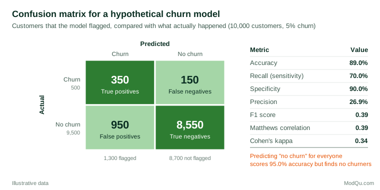
Metrics from the confusion matrix
Accuracy and its trap
Accuracy is the share of all cases classified correctly: (TP + TN) ÷ N. In the example it is (350 + 8,550) ÷ 10,000 = 89.0%. That sounds respectable until one notices that a "model" which predicts that nobody will churn is right 95.0% of the time, because 95% of customers stay. When one class is rare, accuracy mostly measures how well the model recognises the common class, and it can reward a model that never finds the cases the business actually cares about. For this reason accuracy should rarely be the main metric for imbalanced outcomes such as churn, fraud or purchase (He & Garcia, 2009).
Recall, specificity and precision
Three rates describe the model's behaviour more usefully.
- Recall, also called sensitivity or the true positive rate, is TP ÷ (TP + FN): the share of actual churners the model finds. Here 350 ÷ 500 = 70.0%.
- Specificity, or the true negative rate, is TN ÷ (TN + FP): the share of loyal customers correctly left alone. Here 8,550 ÷ 9,500 = 90.0%. Its complement, 10%, is the false positive rate.
- Precision, or positive predictive value, is TP ÷ (TP + FP): the share of flagged customers who really churn. Here 350 ÷ 1,300 = 26.9%.
The low precision is the key business fact. Even with 90% specificity, the 9,500 loyal customers produce more false alarms than the 500 churners produce true alarms, so roughly three of every four retention offers would go to customers who were not going to leave. Recall and specificity do not depend on the share of positives in the data; precision does.
Single-number summaries
Several metrics combine the four counts into one figure. The F1 score is the harmonic mean of precision and recall, 2 × precision × recall ÷ (precision + recall), here 0.39. It ignores true negatives, which is convenient when they are uninteresting but means it can change markedly when the class balance changes (Sokolova & Lapalme, 2009).
The Matthews correlation coefficient (MCC), first proposed for comparing predicted and observed protein structures (Matthews, 1975), is the correlation between predicted and actual classes:
MCC = (TP × TN − FP × FN) ÷ √[(TP + FP)(TP + FN)(TN + FP)(TN + FN)]
It ranges from −1 to +1, with 0 for a classifier no better than chance, and it is high only when the model does well on both classes. Chicco and Jurman (2020) argue that it is more informative than accuracy and F1 for binary problems, especially imbalanced ones. In the example MCC is 0.39.
Cohen's kappa compares observed agreement with the agreement expected by chance from the marginal totals (Cohen, 1960). Here it is 0.34. Balanced accuracy, the average of recall and specificity, is 80.0%, and Youden's index, recall + specificity − 1, is 0.60 (Youden, 1950). None is universally best, so report the confusion matrix itself alongside one or two summaries.
Threshold-free evaluation
ROC curves and AUC
Every metric above depends on the threshold. Lowering the threshold flags more customers, raising recall but also the false positive rate. The receiver operating characteristic (ROC) curve plots the true positive rate against the false positive rate for every possible threshold (Fawcett, 2006). A model with no skill follows the diagonal; a perfect model hugs the top-left corner.
The area under the ROC curve (AUC, also called the c statistic) summarises the whole curve in one number between 0.5 and 1. It has a convenient interpretation: it is the probability that a randomly chosen positive case receives a higher score than a randomly chosen negative case (Hanley & McNeil, 1982). The model in Figure 2 has an AUC of 0.90. Because two models scored on the same test cases produce correlated AUCs, comparisons should use a paired method such as that of DeLong et al. (1988) rather than treating the two estimates as independent.
AUC measures only how well the scores rank cases. It says nothing about whether the probabilities are accurate, and it averages over thresholds that may be irrelevant in practice: a retention team that can contact only 5% of customers cares about the far left of the curve, not the whole of it. Hand (2009) also shows that AUC implicitly weights misclassification costs differently for different classifiers, and proposes an alternative, the H measure.
Precision-recall curves
Because the ROC curve is built from rates within each actual class, it is unaffected by the share of positives (Fawcett, 2006). That is a strength when the base rate varies, but a weakness when positives are rare, because the curve can look excellent while precision is poor. The precision-recall curve plots precision against recall across thresholds, and its summary, average precision, is the area beneath it. For a model with no skill, precision equals the share of positives, so the baseline is low when positives are rare. Saito and Rehmsmeier (2015) show that precision-recall plots are more informative than ROC plots for evaluating classifiers on imbalanced data.
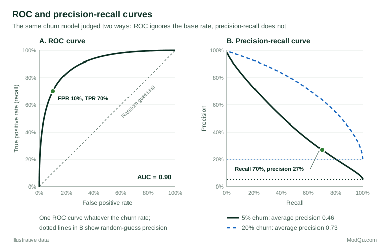
Figure 2 makes the contrast visible. The model's AUC of 0.90 would be the same whether 5% or 20% of customers churned. Its average precision, by contrast, is 0.46 at a 5% churn rate and 0.73 at 20%. Neither number is wrong: AUC describes the model's ability to rank, while the precision-recall curve describes what a business would experience when acting on its flags in a particular population.
Probability quality: calibration and the Brier score
When decisions depend on the predicted probabilities themselves, for example to estimate how many customers will churn next quarter or to compute the expected value of an offer, ranking is not enough. The probabilities must also be calibrated: among customers given a 20% churn probability, about 20% should actually churn. Van Calster et al. (2019) call poor calibration the "Achilles heel" of predictive analytics, because a model with a good AUC can still give probabilities that are systematically too high or too low, leading to poor decisions. Calibration is checked with a calibration plot of observed rates against predicted probabilities, grouped or smoothed, ideally on new data.
The Brier score is the mean squared difference between the predicted probability and the actual outcome coded 0 or 1 (Brier, 1950). Lower is better, and it rewards both discrimination and calibration. Its scale depends on the base rate: a model that predicts 5% for every customer in the example scores 0.05 × 0.95 = 0.0475, so a useful model must do clearly better than that. Steyerberg et al. (2010) recommend reporting overall performance (such as the Brier score), discrimination (such as AUC) and calibration together, because each captures something the others miss.
Choosing a threshold
The threshold should follow from the consequences of each kind of error, not from habit. The default of 0.5 makes sense only when the two errors cost the same and the classes are roughly balanced. If calibrated probabilities are available, decision theory gives a simple rule: flag a case when its probability exceeds
p* = CFP ÷ (CFP + CFN)
where CFP is the cost of a false alarm and CFN the cost of a missed positive. In the churn example, suppose (hypothetically) a retention offer costs $10 per customer contacted and a missed churner who could have been saved costs $90 in lost margin. Then p* = 10 ÷ 100 = 0.10, a much lower threshold than 0.5. With the hypothetical model, a threshold that achieves 90% recall would flag 2,850 loyal customers and reach precision of only 13.6%, which is acceptable if offers are cheap and losses are large, and wasteful if they are not.
Youden's index, by contrast, treats the two error rates as equally important. Decision curve analysis plots the net benefit of acting on the model across a range of threshold probabilities and compares it with the simple strategies of acting on everyone or no one (Vickers & Elkin, 2006):
Net benefit = TP ÷ N − (FP ÷ N) × pt ÷ (1 − pt)
where pt is the threshold probability. A model is worth using at a given threshold only if its net benefit beats both default strategies.
Imbalanced classes
Rare outcomes are the norm in business data: purchase after an advertisement, fraud, complaints, cancellation in a given month. He and Garcia (2009) review the main responses. Resampling methods either under-sample the common class or over-sample the rare one; SMOTE creates synthetic minority cases by interpolating between neighbouring minority examples (Chawla et al., 2002). Cost-sensitive learning instead weights errors on the rare class more heavily during training.
These techniques can improve recall for a given model, but they change the class balance the model sees, so the resulting probabilities are no longer calibrated to the real population. If probabilities are needed, it is often better to train on the natural data, evaluate with precision-recall and calibration, and handle the imbalance through the threshold. Resampling must also be done only inside the training data; synthetic cases that leak into the test set inflate every metric.
More than two classes
For problems with three or more classes, such as assigning respondents to segments, the confusion matrix becomes a k × k table. Per-class precision and recall are combined either by macro-averaging, which gives every class equal weight, or by micro-averaging, which pools all decisions and so gives large classes more influence (Sokolova & Lapalme, 2009). Macro-averages reveal poor performance on small classes, and the full matrix shows which classes are confused.
Practical guidance for survey and business data
- Start from the decision. Ask who will act on the model's output, what each type of error costs, and how many cases can be acted on. Choose metrics that reflect that use, such as precision among the top 5% of scores for a campaign with limited capacity.
- Report a baseline. Compare every model with the trivial rule of predicting the majority class and with a simple logistic regression. A complex model that barely beats them may not be worth its maintenance cost.
- Evaluate on new data in the right population. Use a held-out test set or cross-validation, split by time if the model will predict future behaviour, and make sure the test population has the same base rate as the population where the model will be used.
- Account for survey weights. Unweighted metrics describe the sample, not the population; use weighted counts where the population view matters.
Common mistakes
- Reporting accuracy alone for an imbalanced outcome.
- Treating AUC as a measure of probability accuracy. A model can rank perfectly and still be badly miscalibrated.
- Using the default threshold of 0.5 without considering costs.
- Choosing the threshold, or the model, on the test set and then reporting the test-set performance as an unbiased estimate.
- Rebalancing the classes and then using the model's outputs as if they were real-world probabilities.
Key takeaways
Classifiers, from logistic regression to boosted trees, produce scores that become decisions only through a threshold. Evaluate the scores with ROC and precision-recall curves, and check calibration and the Brier score if probabilities will be used directly. Evaluate the decisions with the confusion matrix and metrics such as recall, precision and MCC that are not fooled by class imbalance. Above all, set the threshold and choose the headline metric according to the costs of the business decision.
References
Breiman, L. (2001). Random forests. Machine Learning, 45(1), 5–32. https://doi.org/10.1023/A:1010933404324
Brier, G. W. (1950). Verification of forecasts expressed in terms of probability. Monthly Weather Review, 78(1), 1–3. https://doi.org/10.1175/1520-0493(1950)078<0001:VOFEIT>2.0.CO;2
Chawla, N. V., Bowyer, K. W., Hall, L. O., & Kegelmeyer, W. P. (2002). SMOTE: Synthetic minority over-sampling technique. Journal of Artificial Intelligence Research, 16, 321–357. https://doi.org/10.1613/jair.953
Chicco, D., & Jurman, G. (2020). The advantages of the Matthews correlation coefficient (MCC) over F1 score and accuracy in binary classification evaluation. BMC Genomics, 21, Article 6. https://doi.org/10.1186/s12864-019-6413-7
Cohen, J. (1960). A coefficient of agreement for nominal scales. Educational and Psychological Measurement, 20(1), 37–46. https://doi.org/10.1177/001316446002000104
Cortes, C., & Vapnik, V. (1995). Support-vector networks. Machine Learning, 20(3), 273–297. https://doi.org/10.1007/BF00994018
DeLong, E. R., DeLong, D. M., & Clarke-Pearson, D. L. (1988). Comparing the areas under two or more correlated receiver operating characteristic curves: A nonparametric approach. Biometrics, 44(3), 837–845. https://doi.org/10.2307/2531595
Fawcett, T. (2006). An introduction to ROC analysis. Pattern Recognition Letters, 27(8), 861–874. https://doi.org/10.1016/j.patrec.2005.10.010
Friedman, J. H. (2001). Greedy function approximation: A gradient boosting machine. The Annals of Statistics, 29(5), 1189–1232. https://doi.org/10.1214/aos/1013203451
Hand, D. J. (2009). Measuring classifier performance: A coherent alternative to the area under the ROC curve. Machine Learning, 77(1), 103–123. https://doi.org/10.1007/s10994-009-5119-5
Hanley, J. A., & McNeil, B. J. (1982). The meaning and use of the area under a receiver operating characteristic (ROC) curve. Radiology, 143(1), 29–36. https://doi.org/10.1148/radiology.143.1.7063747
Hastie, T., Tibshirani, R., & Friedman, J. (2009). The elements of statistical learning: Data mining, inference, and prediction (2nd ed.). Springer. https://doi.org/10.1007/978-0-387-84858-7
He, H., & Garcia, E. A. (2009). Learning from imbalanced data. IEEE Transactions on Knowledge and Data Engineering, 21(9), 1263–1284. https://doi.org/10.1109/TKDE.2008.239
Hosmer, D. W., Jr., Lemeshow, S., & Sturdivant, R. X. (2013). Applied logistic regression (3rd ed.). Wiley. https://doi.org/10.1002/9781118548387
James, G., Witten, D., Hastie, T., & Tibshirani, R. (2021). An introduction to statistical learning: With applications in R (2nd ed.). Springer. https://doi.org/10.1007/978-1-0716-1418-1
Matthews, B. W. (1975). Comparison of the predicted and observed secondary structure of T4 phage lysozyme. Biochimica et Biophysica Acta (BBA) - Protein Structure, 405(2), 442–451. https://doi.org/10.1016/0005-2795(75)90109-9
Saito, T., & Rehmsmeier, M. (2015). The precision-recall plot is more informative than the ROC plot when evaluating binary classifiers on imbalanced datasets. PLOS ONE, 10(3), Article e0118432. https://doi.org/10.1371/journal.pone.0118432
Sokolova, M., & Lapalme, G. (2009). A systematic analysis of performance measures for classification tasks. Information Processing & Management, 45(4), 427–437. https://doi.org/10.1016/j.ipm.2009.03.002
Steyerberg, E. W., Vickers, A. J., Cook, N. R., Gerds, T., Gonen, M., Obuchowski, N., Pencina, M. J., & Kattan, M. W. (2010). Assessing the performance of prediction models: A framework for traditional and novel measures. Epidemiology, 21(1), 128–138. https://doi.org/10.1097/EDE.0b013e3181c30fb2
Van Calster, B., McLernon, D. J., van Smeden, M., Wynants, L., & Steyerberg, E. W. (2019). Calibration: The Achilles heel of predictive analytics. BMC Medicine, 17, Article 230. https://doi.org/10.1186/s12916-019-1466-7
Vickers, A. J., & Elkin, E. B. (2006). Decision curve analysis: A novel method for evaluating prediction models. Medical Decision Making, 26(6), 565–574. https://doi.org/10.1177/0272989X06295361
Youden, W. J. (1950). Index for rating diagnostic tests. Cancer, 3(1), 32–35. https://doi.org/10.1002/1097-0142(1950)3:1<32::AID-CNCR2820030106>3.0.CO;2-3