
Statistics · Causal inference
Causal Inference: From Association to Cause
What it means to say one thing causes another, why simple comparisons mislead, and how experiments, natural experiments and careful adjustment turn associations in business data into credible causal estimates.
Most of the questions that matter in business are causal. Does the loyalty programme make customers spend more, or do big spenders simply join it? Would a price cut raise revenue? Did the new onboarding process reduce churn, or did churn fall for some other reason? Data can show that two things move together. Deciding whether one produces the other is a different and harder task, and it has its own branch of statistics: causal inference.
A companion article on spurious relationships sets out the many ways an association can arise without a causal link. This article takes the next step. It explains what a causal effect is in precise terms, why the obvious comparison usually gets it wrong, and which designs and methods allow analysts to move, with stated assumptions, from association to cause.
What a causal effect is
The modern definition of a causal effect is built on counterfactuals: what would have happened under a different course of action. The idea was written down for agricultural experiments by Jerzy Neyman in 1923 (Splawa-Neyman et al., 1990) and extended to observational studies by Rubin (1974). It is now known as the potential outcomes framework.
Imagine a customer, Ana, who is offered a loyalty programme. She has two potential outcomes: her annual spend if she joins, written Y(1), and her annual spend if she does not, written Y(0). The causal effect of the programme for Ana is the difference between them:
individual effect = Yi(1) − Yi(0)
The catch is obvious once stated. Ana either joins or she does not, so only one of her two potential outcomes is ever observed. Holland (1986) called this the fundamental problem of causal inference: individual causal effects can never be seen directly. Every causal analysis is therefore a way of filling in the missing half of the data with something credible.
Because individual effects are hidden, analysts usually target averages. The average treatment effect (ATE) is the mean of the individual effects across the population:
ATE = E[Y(1) − Y(0)] = E[Y(1)] − E[Y(0)]
A related quantity, the average treatment effect on the treated (ATT), averages only over those who actually received the treatment, such as customers who joined. The two can differ, and choosing between them is a business decision as much as a statistical one. A manager deciding whether to keep a programme for current members needs the ATT; one deciding whether to enrol everyone needs the ATE (Imbens & Rubin, 2015).
Holland (1986) also stressed a practical point: a causal question needs a well-defined intervention. "What is the effect of joining the programme?" can be answered, because joining is something a customer could do or not do. "What is the effect of being a millennial?" is much harder to pin down, because there is no clear alternative version of the same customer to compare against.
Why the obvious comparison misleads
The obvious way to estimate the effect of the loyalty programme is to compare the average spend of members with that of non-members. Potential outcomes show exactly what this comparison measures. With a little algebra, the observed difference splits into two parts (Angrist & Pischke, 2009):
observed difference = ATT + selection bias
Here selection bias is the difference between what members would have spent without the programme and what non-members actually spent. It is zero only if, absent the programme, the two groups would have spent the same.
A worked example
Suppose a hypothetical retailer finds that loyalty members spend $412 a year on average and non-members $280. The naive difference is $132, and a dashboard might report that "the programme adds $132 per customer". But customers who choose to join are not a random slice of the customer base. They already shop frequently, which is why the programme appeals to them. Suppose, again hypothetically, that the members would have spent $350 a year even without the programme. Then the true effect on members is $412 − $350 = $62, and the remaining $70 of the gap is selection bias: the members were bigger spenders all along.
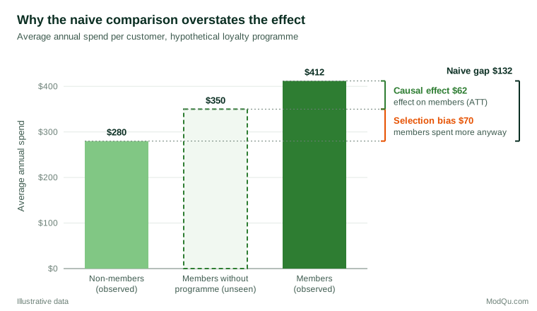
The difficulty is that the $350 in Figure 1 is invisible in the data. Every method of causal inference is, in effect, a strategy for estimating that missing bar.
Three assumptions behind every causal estimate
Whatever method is used, a causal estimate from data rests on a small set of assumptions. They are usually stated as follows (Imbens & Rubin, 2015; Morgan & Winship, 2014).
Exchangeability (no unmeasured confounding). The treated and untreated groups must be comparable in their potential outcomes, either overall or after accounting for measured variables. In the example, members and non-members with the same purchase history, tenure and region must have the same expected spend in the absence of the programme. This assumption cannot be tested from the data alone. It rests on knowledge of how people came to be treated.
Positivity (overlap). Every kind of customer in the analysis must have some chance of receiving each treatment. If no customer with fewer than three purchases a year ever joins, the data hold no information about the programme's effect on infrequent shoppers, and any estimate for them is an extrapolation.
Consistency and no interference. The treatment must be well defined, so that "joining" means the same thing for everyone, and one customer's treatment must not change another's outcome. Rubin called the combination of these conditions the stable unit treatment value assumption. Referral schemes, social media campaigns and marketplace pricing often break it, because one customer's treatment spills over to others.
Drawing the causal story: directed acyclic graphs
Deciding which variables make the groups exchangeable requires a model of how the variables affect one another. Directed acyclic graphs (DAGs) provide one. Each variable is a node and each arrow is an assumed direct causal effect. The graph encodes the analyst's knowledge, and simple rules then show which variables must be adjusted for and which must be left alone (Pearl, 2009; Greenland et al., 1999).
The most useful of these rules, the back-door criterion, says that a set of variables is sufficient for adjustment if it blocks every non-causal path from treatment to outcome that starts with an arrow into the treatment, and contains no variable that is itself an effect of the treatment. In plain terms: adjust for common causes, but not for consequences. In the loyalty example, past purchase frequency affects both joining and future spend, so it belongs in the adjustment set. Number of reward points redeemed is a consequence of joining and does not.
DAGs have two virtues for applied work. They force assumptions into the open, where colleagues can challenge them, and they guard against the instinct to "control for everything", which can introduce bias rather than remove it (Rohrer, 2018). The companion article on confounding works through these choices in detail.
Strategies for identifying causal effects
Methods for causal inference differ mainly in how they argue that the comparison groups are exchangeable. They fall into three broad families.
1. Randomise the treatment
In a randomised experiment, chance decides who is treated. The groups then differ only by chance in everything that existed before treatment, measured or not, and the simple difference in means is an unbiased estimate of the average effect. Fisher (1935) set out the logic of randomisation for agricultural and laboratory experiments, and it underpins today's clinical trials and online A/B tests. Randomisation is the subject of a separate article in this series. Its great strength is that the exchangeability assumption is guaranteed by design rather than argued from background knowledge.
2. Find variation that is as good as random
When an experiment is impossible, analysts look for situations in which treatment was assigned by something unrelated to the outcome. These natural experiments and quasi-experiments include several well-established designs.
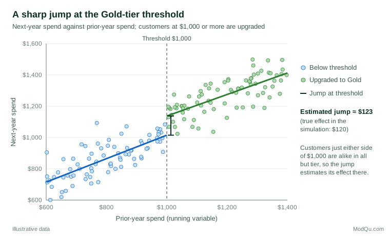
- Regression discontinuity. Treatment switches on at a threshold of some running variable, such as a test score or a spending level. Units just above and just below the threshold are nearly identical, so any jump in the outcome at the threshold estimates the effect there. Thistlethwaite and Campbell (1960) introduced the design to study the effect of public recognition of high-scoring students on their later plans.
- Instrumental variables. An instrument shifts the chance of treatment but affects the outcome only through the treatment. Angrist et al. (1996) showed that, under clearly stated assumptions, an instrumental variable estimate recovers the average effect for "compliers", those whose treatment status the instrument actually changed, using the Vietnam-era draft lottery as their example.
- Difference-in-differences. The change over time in a treated group is compared with the change in an untreated group over the same period. The design assumes that, without the treatment, both groups would have followed parallel trends (Angrist & Pischke, 2009).
- Synthetic control and time-series methods. When only one unit is treated, such as a single region that launches a campaign, a weighted combination of untreated units can be built to mimic its pre-treatment path (Abadie et al., 2010). Bayesian structural time-series models apply a similar idea to forecast what a treated series would have done without the intervention (Brodersen et al., 2015).
Figure 2 shows a hypothetical regression discontinuity. A retailer upgrades every customer who spent $1,000 or more last year to a Gold tier. Next-year spend rises smoothly with prior spend, but at the threshold it jumps. Because customers who spent $990 and $1,010 are alike in almost every respect, the size of the jump estimates the effect of the Gold tier for customers near the threshold.
The price of these designs is that each answers a narrower question than an experiment. A regression discontinuity estimates the effect at the threshold, not for all customers. An instrumental variable estimates it for compliers. Each also rests on its own assumption, such as no manipulation of the running variable or parallel trends, which should be checked as far as the data allow.
3. Adjust for measured confounders
The most common approach in business analytics is to compare treated and untreated units that are similar on measured characteristics, using regression, stratification, matching or weighting. Rosenbaum and Rubin (1983) showed that, if exchangeability holds given a set of covariates, it also holds given a single summary of them, the propensity score, which is the probability of treatment given the covariates. Matching or weighting on that score can balance many covariates at once.
These methods are only as good as the list of measured confounders. They remove the bias from variables that are recorded and correctly modelled, and do nothing about those that are not. Their credibility therefore depends heavily on the causal reasoning that went into choosing the covariates.
How far can observational methods be trusted?
Comparisons between experimental and observational estimates of the same effect are sobering. Gordon et al. (2019) analysed 15 large advertising experiments run at Facebook and applied common observational methods to the same campaigns. The observational estimates were often far from the experimental benchmark and tended to overstate the advertising lift, sometimes by a wide margin. Blake et al. (2015) reported a related lesson from eBay. When the company stopped paying for search ads on its own brand name, almost all of the lost traffic arrived through the unpaid search results instead: the customers who clicked brand ads were going to visit anyway. Simple correlations between ad clicks and sales had made the ads look far more valuable than they were.
The lesson is not that observational analysis is useless. Some of the most important causal conclusions in history, such as the link between smoking and lung cancer, were reached without randomisation, by weighing the strength, consistency, timing and dose-response pattern of the evidence (Hill, 1965). The lesson is that observational estimates need explicit assumptions, careful design and honest statements of uncertainty.
Making observational studies more credible
Several practices narrow the gap between observational and experimental evidence.
Emulate a target trial. Before analysing observational data, describe the randomised trial that would ideally answer the question: who is eligible, what treatments are compared, when follow-up starts and what outcome is measured. Then design the observational analysis to mimic it as closely as possible (Hernán & Robins, 2016). This simple step avoids common errors such as comparing customers at different points in their journey, or counting outcomes that occurred before treatment.
Separate design from analysis. Choose the comparison groups and check their balance before looking at the outcomes. This prevents the analysis from being tuned, consciously or not, towards a preferred answer.
Quantify sensitivity to unmeasured confounding. Sensitivity analysis asks how strong an unmeasured confounder would have to be to change the conclusion. The E-value expresses this as the minimum strength of association, on the risk ratio scale, that a confounder would need with both treatment and outcome to explain away an observed risk ratio RR (VanderWeele & Ding, 2017):
E-value = RR + √(RR × (RR − 1))
For an observed risk ratio of 1.5, the E-value is about 2.4: a hidden factor would need to be associated with both treatment and outcome by a risk ratio of at least 2.4 each to remove the effect entirely. Cinelli and Hazlett (2020) offer an equivalent approach for linear regression, expressed in terms of how much variance a confounder would have to explain, and allow comparison with the strongest measured covariates.
Use negative checks. If the "effect" of the loyalty programme also appears in spending from the year before customers joined, the comparison is picking up selection rather than causation.
Causal inference with survey and business data
Survey data raise particular challenges for causal questions.
- Timing is often unclear. A cross-sectional survey measures attitudes and behaviour at the same moment, so it is hard to know which came first. Satisfaction may drive loyalty, but loyal customers may also report higher satisfaction. Panel designs, which follow the same respondents over time, and questions that date events help to establish order.
- Driver analysis is associational. Key-driver models that relate overall satisfaction to attribute ratings describe patterns in the data. They do not show that improving an attribute would raise satisfaction by the estimated amount.
- Survey experiments are cheap and powerful. Randomly varying a question wording, price point, concept description or message between respondents creates a true experiment within the survey, with the internal validity that randomisation brings.
- Sample selection is itself a causal problem. Inferring from a nonprobability sample to a population requires assumptions that parallel those of causal inference: exchangeability given the weighting variables, positivity and correct composition (Mercer et al., 2017). The same discipline of stating assumptions applies to both.
Common mistakes
- Reading every regression coefficient as causal. A model built to estimate one effect does not give valid causal estimates for the other covariates in it. Westreich and Greenland (2013) call this the "Table 2 fallacy".
- Hiding causal aims behind cautious wording. Reports often describe "associations" while recommending action as if the effect were causal. Hernán (2018) argues that it is better to state the causal question openly and then be explicit about the assumptions needed to answer it.
- Adjusting for consequences of the treatment. Controlling for variables that the treatment itself changes removes part of the effect being measured.
- Ignoring overlap. Estimates for customer types that rarely or never receive the treatment are extrapolations from a model, not evidence.
- Confusing statistical significance with causal credibility. A very small p-value says nothing about whether the comparison groups were exchangeable.
Key takeaways
A causal effect is a comparison between what happened and what would have happened under a different course of action. Because only one of these is ever observed for each unit, causal inference always relies on assumptions about the missing counterfactual. Randomised experiments make those assumptions true by design. Natural experiments and quasi-experimental designs find situations where they are plausible. Adjustment methods such as regression and propensity scores make them credible only when the right confounders are measured. For business and survey analysts, the practical habits are to define the intervention and the target population, draw the causal assumptions as a diagram, choose the strongest feasible design, check balance and overlap, test sensitivity to hidden confounding and report causal claims with the assumptions that support them.
References
Abadie, A., Diamond, A., & Hainmueller, J. (2010). Synthetic control methods for comparative case studies: Estimating the effect of California's tobacco control program. Journal of the American Statistical Association, 105(490), 493–505. https://doi.org/10.1198/jasa.2009.ap08746
Angrist, J. D., Imbens, G. W., & Rubin, D. B. (1996). Identification of causal effects using instrumental variables. Journal of the American Statistical Association, 91(434), 444–455. https://doi.org/10.1080/01621459.1996.10476902
Angrist, J. D., & Pischke, J.-S. (2009). Mostly harmless econometrics: An empiricist's companion. Princeton University Press. https://doi.org/10.1515/9781400829828
Blake, T., Nosko, C., & Tadelis, S. (2015). Consumer heterogeneity and paid search effectiveness: A large-scale field experiment. Econometrica, 83(1), 155–174. https://doi.org/10.3982/ECTA12423
Brodersen, K. H., Gallusser, F., Koehler, J., Rémy, N., & Scott, S. L. (2015). Inferring causal impact using Bayesian structural time-series models. The Annals of Applied Statistics, 9(1), 247–274. https://doi.org/10.1214/14-AOAS788
Cinelli, C., & Hazlett, C. (2020). Making sense of sensitivity: Extending omitted variable bias. Journal of the Royal Statistical Society Series B: Statistical Methodology, 82(1), 39–67. https://doi.org/10.1111/rssb.12348
Fisher, R. A. (1935). The design of experiments. Oliver and Boyd.
Gordon, B. R., Zettelmeyer, F., Bhargava, N., & Chapsky, D. (2019). A comparison of approaches to advertising measurement: Evidence from big field experiments at Facebook. Marketing Science, 38(2), 193–225. https://doi.org/10.1287/mksc.2018.1135
Greenland, S., Pearl, J., & Robins, J. M. (1999). Causal diagrams for epidemiologic research. Epidemiology, 10(1), 37–48. https://doi.org/10.1097/00001648-199901000-00008
Hernán, M. A. (2018). The C-word: Scientific euphemisms do not improve causal inference from observational data. American Journal of Public Health, 108(5), 616–619. https://doi.org/10.2105/AJPH.2018.304337
Hernán, M. A., & Robins, J. M. (2016). Using big data to emulate a target trial when a randomized trial is not available. American Journal of Epidemiology, 183(8), 758–764. https://doi.org/10.1093/aje/kwv254
Hill, A. B. (1965). The environment and disease: Association or causation? Proceedings of the Royal Society of Medicine, 58(5), 295–300. https://doi.org/10.1177/003591576505800503
Holland, P. W. (1986). Statistics and causal inference. Journal of the American Statistical Association, 81(396), 945–960. https://doi.org/10.1080/01621459.1986.10478354
Imbens, G. W., & Rubin, D. B. (2015). Causal inference for statistics, social, and biomedical sciences: An introduction. Cambridge University Press. https://doi.org/10.1017/CBO9781139025751
Mercer, A. W., Kreuter, F., Keeter, S., & Stuart, E. A. (2017). Theory and practice in nonprobability surveys: Parallels between causal inference and survey inference. Public Opinion Quarterly, 81(S1), 250–271. https://doi.org/10.1093/poq/nfw060
Morgan, S. L., & Winship, C. (2014). Counterfactuals and causal inference: Methods and principles for social research (2nd ed.). Cambridge University Press. https://doi.org/10.1017/CBO9781107587991
Pearl, J. (2009). Causality: Models, reasoning, and inference (2nd ed.). Cambridge University Press. https://doi.org/10.1017/CBO9780511803161
Rohrer, J. M. (2018). Thinking clearly about correlations and causation: Graphical causal models for observational data. Advances in Methods and Practices in Psychological Science, 1(1), 27–42. https://doi.org/10.1177/2515245917745629
Rosenbaum, P. R., & Rubin, D. B. (1983). The central role of the propensity score in observational studies for causal effects. Biometrika, 70(1), 41–55. https://doi.org/10.1093/biomet/70.1.41
Rubin, D. B. (1974). Estimating causal effects of treatments in randomized and nonrandomized studies. Journal of Educational Psychology, 66(5), 688–701. https://doi.org/10.1037/h0037350
Splawa-Neyman, J., Dabrowska, D. M., & Speed, T. P. (1990). On the application of probability theory to agricultural experiments. Essay on principles. Section 9. Statistical Science, 5(4), 465–472. https://doi.org/10.1214/ss/1177012031
Thistlethwaite, D. L., & Campbell, D. T. (1960). Regression-discontinuity analysis: An alternative to the ex post facto experiment. Journal of Educational Psychology, 51(6), 309–317. https://doi.org/10.1037/h0044319
VanderWeele, T. J., & Ding, P. (2017). Sensitivity analysis in observational research: Introducing the E-value. Annals of Internal Medicine, 167(4), 268–274. https://doi.org/10.7326/M16-2607
Westreich, D., & Greenland, S. (2013). The Table 2 fallacy: Presenting and interpreting confounder and modifier coefficients. American Journal of Epidemiology, 177(4), 292–298. https://doi.org/10.1093/aje/kws412