
Research · Research design
Quasi-Experimental Designs When Randomisation Is Not Possible
The main quasi-experimental designs used when random assignment is impossible (comparison groups, difference-in-differences, interrupted time series, regression discontinuity, matching and synthetic controls), how each approximates an experiment, and what assumptions it rests on.
Randomised experiments are the most reliable way to establish cause and effect, but they are often impossible. A company cannot randomly assign some cities to a new minimum wage, some stores to a fire or some customers to a recession. Even when random assignment is technically possible, it may be too expensive, too slow or unacceptable to the people involved. Quasi-experimental designs are the family of methods used in these situations. They study an intervention that the researcher did not randomly assign and use design features, rather than chance, to rule out alternative explanations. This article explains the main designs, how each tries to recover the logic of an experiment, and the assumptions on which each one depends.
What a quasi-experiment lacks
Campbell and Stanley (1963) introduced the term to describe designs that have a treatment, outcome measures and some form of comparison, but no random assignment. Without randomisation, the groups being compared may differ before the treatment begins, and those differences rather than the treatment may explain any difference in outcomes. Cook and Campbell (1979) and Shadish et al. (2002) catalogued these alternative explanations as threats to internal validity: selection (the groups were different to begin with), history (something else happened at the same time), maturation (the groups were changing anyway), regression to the mean (units were chosen because of unusually high or low scores) and others.
The strategy of quasi-experimental design is to anticipate which threats are plausible in a given study and add design elements that make each one less likely. Shadish et al. (2002) stress that this is a matter of reasoning about the specific case, not of applying a formula.
Non-equivalent comparison groups
The simplest design compares a group that received the treatment with a group that did not, measuring both before and after. A retailer introduces a new store layout in its Ottawa branches and compares their sales with branches in Winnipeg that kept the old layout. The pre-treatment measurement shows how similar the groups were before the change. If they were similar and moved together until the change, a divergence afterwards is more convincing evidence of an effect.
The weakness is selection. Branches chosen for a new layout may have been chosen because their managers were enthusiastic, or because sales were already falling, and either reason could affect later sales.
Difference-in-differences
Difference-in-differences formalises the comparison group design. It calculates the change in the outcome for the treated group, subtracts the change for the comparison group, and treats the remainder as the effect. The comparison group's change stands in for what would have happened to the treated group without the treatment.
Card and Krueger (1994) used this design in a well-known study of the minimum wage. When New Jersey raised its minimum wage in 1992, they surveyed fast-food restaurants in New Jersey and in neighbouring eastern Pennsylvania, where the minimum wage did not change, before and after the increase. Comparing the change in employment across the two states allowed them to separate the effect of the policy from regional trends affecting both.
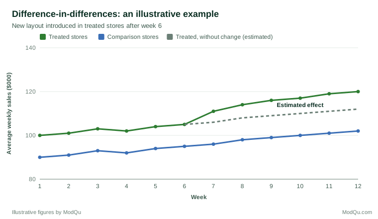
The key assumption is parallel trends: without the treatment, both groups would have followed the same path. It cannot be tested directly, because the treated group's untreated path is never observed, but it can be checked indirectly by looking at whether the groups moved together over several periods before the treatment (Angrist & Pischke, 2009).
Interrupted time series
When there is no obvious comparison group, an interrupted time series uses the treated group's own history. The outcome is measured at many points before and after the intervention, and the pre-intervention trend is projected forward to estimate what would have happened. A change in level or slope at the moment of intervention is evidence of an effect. Lopez Bernal et al. (2017) describe how the design is used to evaluate public health policies, such as smoking bans, where outcomes such as hospital admissions are recorded routinely.
The main threat is history: another event occurring at the same time as the intervention. Long series, a sharp and well-defined start date, and a comparison series unaffected by the intervention all help rule this out. Seasonal patterns must also be modelled, so that a normal December peak is not mistaken for the effect of a November campaign.
Regression discontinuity
Many treatments are assigned by a rule based on a score: students above a certain grade receive a scholarship, customers who spend more than a threshold receive premium status, applicants below an income limit qualify for support. Thistlethwaite and Campbell (1960) recognised that this creates an opportunity. People just above and just below the cut-off are likely to be very similar in every respect except treatment, so comparing them approximates a randomised experiment in the neighbourhood of the threshold.
Lee and Lemieux (2010) showed that a regression discontinuity design gives credible estimates when people cannot precisely control which side of the cut-off they fall on. If customers can easily adjust their spending to just pass a loyalty threshold, those just above may differ systematically from those just below, and the design loses its force. A practical check is to look for an unusual bunching of cases just above the threshold. The estimate applies only to units near the cut-off, which may not be the group a decision-maker cares about most.
Matching and propensity scores
When treated and untreated units differ on measured characteristics, matching pairs each treated unit with one or more similar untreated units. Rosenbaum and Rubin (1983) showed that matching on the propensity score, the estimated probability of receiving the treatment given observed characteristics, can balance many characteristics at once.
Matching can only balance what is measured. If customers who joined a loyalty programme differ from non-members in motivation that the data do not capture, matched comparisons will still be biased. LaLonde (1986) gave a sobering demonstration: when he compared the results of a randomised job training experiment with estimates from several non-experimental methods applied to the same programme, many of the non-experimental estimates were far from the experimental benchmark.
Synthetic controls
When the treated unit is a single region, organisation or market, a synthetic control builds a comparison from a weighted combination of untreated units chosen so that, together, they reproduce the treated unit's pre-treatment path. Abadie et al. (2010) used the method to estimate the effect of California's 1988 tobacco control programme on cigarette consumption, constructing a "synthetic California" from other states. The method makes the choice of comparison transparent, but it relies on a good pre-treatment fit and on no other major event affecting the treated unit alone.
How well do quasi-experiments work?
Studies that compare quasi-experimental estimates with randomised benchmarks suggest the answer depends on the design. Cook et al. (2008) reviewed such within-study comparisons and found that regression discontinuity designs generally reproduced experimental results, and that other designs did so when the comparison group was well chosen and the process that selected units for treatment was understood and measured. Designs that rely on statistical adjustment alone, with an arbitrary comparison group, were the least reliable.
Choosing a design
The choice usually depends on how the treatment was assigned. If it followed a threshold rule, regression discontinuity is the natural choice. If it began at a known date in some places and not others, difference-in-differences fits. If it affected everyone at once, an interrupted time series is often the only option. If a single unit was treated, a synthetic control may be best. Imbens and Rubin (2015) recommend designing a quasi-experiment as if it were an experiment: define the treatment, the units and the outcome in advance, and settle the comparison before looking at the outcome data.
Whatever the design, the conclusion should be reported with its assumptions. A difference-in-differences result is only as credible as the parallel trends assumption behind it, and readers deserve to see the evidence for that assumption alongside the estimate.
References
Abadie, A., Diamond, A., & Hainmueller, J. (2010). Synthetic control methods for comparative case studies: Estimating the effect of California's tobacco control program. Journal of the American Statistical Association, 105(490), 493–505. https://doi.org/10.1198/jasa.2009.ap08746
Angrist, J. D., & Pischke, J.-S. (2009). Mostly harmless econometrics: An empiricist's companion. Princeton University Press.
Campbell, D. T., & Stanley, J. C. (1963). Experimental and quasi-experimental designs for research. Rand McNally.
Card, D., & Krueger, A. B. (1994). Minimum wages and employment: A case study of the fast-food industry in New Jersey and Pennsylvania. American Economic Review, 84(4), 772–793.
Cook, T. D., & Campbell, D. T. (1979). Quasi-experimentation: Design and analysis issues for field settings. Houghton Mifflin.
Cook, T. D., Shadish, W. R., & Wong, V. C. (2008). Three conditions under which experiments and observational studies produce comparable causal estimates: New findings from within-study comparisons. Journal of Policy Analysis and Management, 27(4), 724–750. https://doi.org/10.1002/pam.20375
Imbens, G. W., & Rubin, D. B. (2015). Causal inference for statistics, social, and biomedical sciences: An introduction. Cambridge University Press. https://doi.org/10.1017/CBO9781139025751
LaLonde, R. J. (1986). Evaluating the econometric evaluations of training programs with experimental data. American Economic Review, 76(4), 604–620.
Lee, D. S., & Lemieux, T. (2010). Regression discontinuity designs in economics. Journal of Economic Literature, 48(2), 281–355. https://doi.org/10.1257/jel.48.2.281
Lopez Bernal, J., Cummins, S., & Gasparrini, A. (2017). Interrupted time series regression for the evaluation of public health interventions: A tutorial. International Journal of Epidemiology, 46(1), 348–355. https://doi.org/10.1093/ije/dyw098
Rosenbaum, P. R., & Rubin, D. B. (1983). The central role of the propensity score in observational studies for causal effects. Biometrika, 70(1), 41–55. https://doi.org/10.1093/biomet/70.1.41
Shadish, W. R., Cook, T. D., & Campbell, D. T. (2002). Experimental and quasi-experimental designs for generalized causal inference. Houghton Mifflin.
Thistlethwaite, D. L., & Campbell, D. T. (1960). Regression-discontinuity analysis: An alternative to the ex post facto experiment. Journal of Educational Psychology, 51(6), 309–317. https://doi.org/10.1037/h0044319