
Research · Literature and evidence
Meta-Analysis: Combining Results Across Studies
How meta-analysis combines results from many studies into an overall estimate, covering effect sizes, weighting, fixed-effect and random-effects models, heterogeneity, forest plots, moderators, publication bias, quality and common misuses.
When many studies have addressed the same question, their results rarely agree exactly. Some find large effects, some small, some none. Reading them one by one invites confusion, or a tally of "positive" and "negative" studies that ignores how large and precise each result was. Meta-analysis is a set of statistical methods for combining the results of several studies into a single estimate, while examining how and why results differ. Glass (1976), who coined the term, described it as the statistical analysis of a large collection of results from individual studies for the purpose of integrating the findings. This article explains how meta-analysis works, how to read its results and where it can mislead.
Origins
Smith and Glass (1977) published one of the first major meta-analyses, combining the results of hundreds of studies of psychotherapy. They found that the average person receiving therapy was better off than about three-quarters of those who did not. The study was influential and controversial. Eysenck (1978) dismissed it as "an exercise in mega-silliness", arguing that combining studies of varying quality produced a meaningless average. The criticism, sometimes summarised as "garbage in, garbage out", remains relevant, and has shaped how careful meta-analyses assess study quality.
Lau et al. (1992) showed the value of meta-analysis with a cumulative meta-analysis of trials of treatments for heart attack. By adding trials one at a time in the order they were published, they showed that the evidence for the benefit of some treatments had been clear years before experts began recommending them in textbooks and reviews. Earlier synthesis could have saved lives.
Effect sizes
To combine studies, their results must be expressed on a common scale. An effect size measures the size of a difference or relationship in a standard form. Common effect sizes include:
- the standardised mean difference, which expresses the difference between two group means in units of standard deviation;
- the correlation coefficient, for relationships between two continuous variables;
- the odds ratio or risk ratio, for binary outcomes such as whether a customer renewed or not.
Cohen (1988) suggested that standardised mean differences of about 0.2, 0.5 and 0.8 could be called small, medium and large, while stressing that these labels were rough conventions and that what counts as important depends on the field. Lipsey and Wilson (2001) explained how to calculate effect sizes from the statistics that studies report, which often requires converting between different measures.
Weighting and pooling
Meta-analysis does not simply average the effect sizes. Larger and more precise studies carry more information, so they receive more weight. The usual approach weights each study by the inverse of its variance, so that studies with smaller standard errors count for more (Borenstein et al., 2009).
There are two main models for pooling. A fixed-effect model assumes that all studies estimate the same true effect, and that differences between them arise only from sampling error. A random-effects model assumes that the true effect varies from study to study, because of differences in populations, settings or methods, and estimates the average of this distribution of effects. DerSimonian and Laird (1986) proposed a widely used method for estimating random-effects models. The comparison below summarises the two.
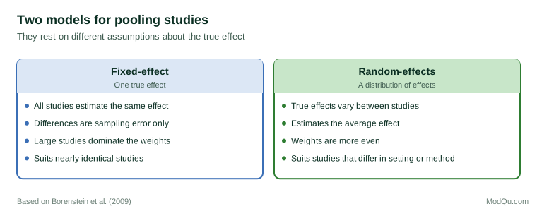
Borenstein et al. (2009) argued that the choice should depend on the assumptions that fit the studies, not on the results of a test. In most social and business research, where studies differ in many ways, the random-effects model is more realistic.
The forest plot
Meta-analyses are usually displayed as a forest plot. Each study is shown as a square at its effect estimate, with a horizontal line showing its confidence interval. The size of the square reflects the study's weight. A diamond at the bottom shows the pooled estimate, with its width showing the confidence interval. A vertical line marks no effect. The chart below shows an illustrative example.
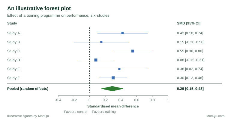
A forest plot shows at a glance whether studies agree, which studies are most influential and how precise the overall estimate is.
Interpreting effect sizes in practice
An effect size is only useful if readers understand what it means. A standardised mean difference of 0.30 is abstract; it becomes meaningful when translated into the units decision-makers use. Lipsey and Wilson (2001) recommended expressing results in familiar terms where possible, such as the percentage improvement in a sales figure, the change in the proportion of customers who renew, or the number of people who would need to receive an intervention for one additional person to benefit. Comparing an effect with the effects of other interventions in the same field is often more informative than comparing it with general benchmarks of small, medium and large (Cohen, 1988). A small effect may be very valuable if the intervention is cheap and reaches many people; a large effect may matter little if the outcome itself is unimportant.
Heterogeneity
Variation in true effects across studies is called heterogeneity. Higgins and Thompson (2002) proposed the I-squared statistic, which describes the percentage of variation across studies that is due to heterogeneity rather than chance. Higgins et al. (2003) suggested that values around 25, 50 and 75 percent could be read as low, moderate and high heterogeneity, while noting that interpretation depends on context.
Heterogeneity matters because the pooled average may not describe any particular setting well. Riley et al. (2011) emphasised that in a random-effects meta-analysis the summary estimate is the average effect, not a single common effect, and recommended reporting a prediction interval showing the range in which the effect in a new setting is likely to fall. IntHout et al. (2016) found that prediction intervals were often much wider than confidence intervals, and that many meta-analyses with a clearly positive average effect had prediction intervals including no effect or harm.
Explaining differences
When heterogeneity is substantial, researchers try to explain it. Subgroup analysis compares pooled effects across groups of studies, such as studies in different countries or using different versions of an intervention. Meta-regression relates effect sizes to study characteristics. Thompson and Higgins (2002) cautioned that meta-regression is observational, since the characteristics are not randomly assigned to studies, that it has low power when there are few studies, and that testing many characteristics risks finding spurious relationships. Planned analyses, specified in a protocol, are more credible than those chosen after looking at the data.
Hunter and Schmidt (2004) developed an approach that corrects effect sizes for artefacts such as measurement error and restricted range before pooling, on the grounds that much apparent variation between studies is due to these artefacts rather than real differences.
Publication bias
Meta-analysis can only combine the studies it finds. If studies with significant or striking results are more likely to be published, the pooled estimate will be too large. Rosenthal (1979) called this the file drawer problem: for every published study, others with null results may sit unpublished in researchers' files.
Several methods help detect and adjust for publication bias. A funnel plot shows each study's effect size against its precision. Without bias, small studies should scatter widely and symmetrically around the average; a gap where small studies with null results should be suggests that such studies are missing. Egger et al. (1997) proposed a regression test for funnel plot asymmetry. Duval and Tweedie (2000) developed the trim and fill method, which estimates how many studies are missing and adjusts the pooled estimate. Simonsohn et al. (2014) proposed p-curve, which examines the distribution of significant p-values to assess whether a set of findings reflects a true effect. Each method has limitations, and asymmetry can arise for reasons other than publication bias, such as smaller studies being done in different populations. No statistical method can fully recover studies that were never published, so the best defence is prevention: searching trial registers, conference abstracts, theses and other grey literature, and contacting researchers for unpublished results. Prospective registration of studies, now required for clinical trials in many countries, makes it easier to find studies that were started but never reported.
Quality and risk of bias
The criticism of Eysenck (1978) still applies: combining biased studies produces a biased estimate, however precise it looks. Careful meta-analyses assess each study's risk of bias, and examine whether results differ between studies at high and low risk. The Cochrane Handbook recommends assessing risk of bias for each study and taking it into account in the synthesis, for example by restricting the main analysis to studies at low risk (Higgins et al., 2019).
Extensions
Several extensions of meta-analysis address particular problems. Individual participant data meta-analysis obtains the raw data from each study rather than the published summary results. This allows consistent analysis across studies, better handling of missing data and more reliable analysis of which people benefit most, though it requires cooperation from the original researchers and much more work. Network meta-analysis compares several interventions at once, combining direct comparisons, such as A against B, with indirect ones, such as A against C and B against C, to estimate how all the options rank. The Cochrane Handbook describes both approaches and the additional assumptions they require (Higgins et al., 2019). In business settings, the same logic underlies the pooling of results from many related experiments, such as a series of tests of website changes, to estimate typical effects and how much they vary.
Carrying out a meta-analysis
A meta-analysis is usually part of a systematic review. The main steps are:
- specify the question and eligibility criteria in a protocol;
- search systematically for all relevant studies, published and unpublished;
- extract effect sizes and their standard errors, and study characteristics;
- assess each study's risk of bias;
- choose a model and pool the effect sizes;
- examine heterogeneity and, where planned, explore its sources;
- assess publication bias and the robustness of results;
- report transparently, following guidelines such as PRISMA 2020 (Page et al., 2021).
Software makes the calculations straightforward. Viechtbauer (2010) described the widely used metafor package for the R environment. Cooper et al. (2019) provide a comprehensive handbook of methods.
Common misuses
Meta-analysis is powerful but can mislead:
- Combining apples and oranges. Pooling studies that measure different things or test different interventions produces an average with no clear meaning.
- Ignoring heterogeneity. Reporting only the pooled estimate hides how much effects vary.
- Ignoring bias. A precise pooled estimate from biased studies is precisely wrong.
- Overinterpreting subgroups. Differences between subgroups found after the fact are often due to chance.
- Treating the pooled estimate as certain. The confidence interval, prediction interval and quality of the evidence all matter.
An applied example
A hypothetical example: a company wants to know how much a type of sales training improves performance. A systematic review finds twelve studies reporting standardised mean differences. A random-effects meta-analysis estimates an average effect of 0.30, with a 95 percent confidence interval from 0.15 to 0.45, indicating a modest positive effect on average. But I-squared is 65 percent, and the prediction interval runs from about −0.10 to 0.70, so in some settings the training may have little or no effect. A subgroup analysis planned in advance shows larger effects when training is followed by coaching. A funnel plot shows some asymmetry, suggesting that small studies with null results may be missing. The company concludes that the training is worth trying, with coaching, and that its effect should be measured locally. The figures are illustrative, but they show how a meta-analysis can inform a decision while revealing its uncertainties.
Conclusion
Meta-analysis combines evidence from many studies, weighting each by its precision, to estimate an overall effect and examine how effects vary. Its results are displayed in forest plots, interpreted with attention to heterogeneity and prediction intervals, and checked for publication bias and study quality. Used carefully, it gives the most precise and complete summary of what a body of research shows. Used carelessly, it can turn weak or biased evidence into a misleadingly confident number.
References
Borenstein, M., Hedges, L. V., Higgins, J. P. T., & Rothstein, H. R. (2009). Introduction to meta-analysis. Wiley. https://doi.org/10.1002/9780470743386
Cohen, J. (1988). Statistical power analysis for the behavioral sciences (2nd ed.). Lawrence Erlbaum Associates.
Cooper, H., Hedges, L. V., & Valentine, J. C. (Eds.). (2019). The handbook of research synthesis and meta-analysis (3rd ed.). Russell Sage Foundation.
DerSimonian, R., & Laird, N. (1986). Meta-analysis in clinical trials. Controlled Clinical Trials, 7(3), 177–188. https://doi.org/10.1016/0197-2456(86)90046-2
Duval, S., & Tweedie, R. (2000). Trim and fill: A simple funnel-plot-based method of testing and adjusting for publication bias in meta-analysis. Biometrics, 56(2), 455–463. https://doi.org/10.1111/j.0006-341X.2000.00455.x
Egger, M., Davey Smith, G., Schneider, M., & Minder, C. (1997). Bias in meta-analysis detected by a simple, graphical test. BMJ, 315(7109), 629–634. https://doi.org/10.1136/bmj.315.7109.629
Eysenck, H. J. (1978). An exercise in mega-silliness. American Psychologist, 33(5), 517. https://doi.org/10.1037/0003-066X.33.5.517.a
Glass, G. V. (1976). Primary, secondary, and meta-analysis of research. Educational Researcher, 5(10), 3–8. https://doi.org/10.3102/0013189X005010003
Higgins, J. P. T., Thomas, J., Chandler, J., Cumpston, M., Li, T., Page, M. J., & Welch, V. A. (Eds.). (2019). Cochrane handbook for systematic reviews of interventions (2nd ed.). Wiley. https://doi.org/10.1002/9781119536604
Higgins, J. P. T., & Thompson, S. G. (2002). Quantifying heterogeneity in a meta-analysis. Statistics in Medicine, 21(11), 1539–1558. https://doi.org/10.1002/sim.1186
Higgins, J. P. T., Thompson, S. G., Deeks, J. J., & Altman, D. G. (2003). Measuring inconsistency in meta-analyses. BMJ, 327(7414), 557–560. https://doi.org/10.1136/bmj.327.7414.557
Hunter, J. E., & Schmidt, F. L. (2004). Methods of meta-analysis: Correcting error and bias in research findings (2nd ed.). SAGE. https://doi.org/10.4135/9781412985031
IntHout, J., Ioannidis, J. P. A., Rovers, M. M., & Goeman, J. J. (2016). Plea for routinely presenting prediction intervals in meta-analysis. BMJ Open, 6(7), Article e010247. https://doi.org/10.1136/bmjopen-2015-010247
Lau, J., Antman, E. M., Jimenez-Silva, J., Kupelnick, B., Mosteller, F., & Chalmers, T. C. (1992). Cumulative meta-analysis of therapeutic trials for myocardial infarction. New England Journal of Medicine, 327(4), 248–254. https://doi.org/10.1056/NEJM199207233270406
Lipsey, M. W., & Wilson, D. B. (2001). Practical meta-analysis. SAGE.
Page, M. J., McKenzie, J. E., Bossuyt, P. M., Boutron, I., Hoffmann, T. C., Mulrow, C. D., Shamseer, L., Tetzlaff, J. M., Akl, E. A., Brennan, S. E., Chou, R., Glanville, J., Grimshaw, J. M., Hróbjartsson, A., Lalu, M. M., Li, T., Loder, E. W., Mayo-Wilson, E., McDonald, S., … Moher, D. (2021). The PRISMA 2020 statement: An updated guideline for reporting systematic reviews. BMJ, 372, Article n71. https://doi.org/10.1136/bmj.n71
Riley, R. D., Higgins, J. P. T., & Deeks, J. J. (2011). Interpretation of random effects meta-analyses. BMJ, 342, Article d549. https://doi.org/10.1136/bmj.d549
Rosenthal, R. (1979). The file drawer problem and tolerance for null results. Psychological Bulletin, 86(3), 638–641. https://doi.org/10.1037/0033-2909.86.3.638
Simonsohn, U., Nelson, L. D., & Simmons, J. P. (2014). P-curve: A key to the file-drawer. Journal of Experimental Psychology: General, 143(2), 534–547. https://doi.org/10.1037/a0033242
Smith, M. L., & Glass, G. V. (1977). Meta-analysis of psychotherapy outcome studies. American Psychologist, 32(9), 752–760. https://doi.org/10.1037/0003-066X.32.9.752
Thompson, S. G., & Higgins, J. P. T. (2002). How should meta-regression analyses be undertaken and interpreted? Statistics in Medicine, 21(11), 1559–1573. https://doi.org/10.1002/sim.1187
Viechtbauer, W. (2010). Conducting meta-analyses in R with the metafor package. Journal of Statistical Software, 36(3), 1–48. https://doi.org/10.18637/jss.v036.i03