
Research · Market and business research
Market Sizing Research: Top-Down and Bottom-Up Methods
How to estimate the size of a market using top-down and bottom-up methods, how to define total, serviceable and obtainable market, how to forecast new markets, and how to check estimates against bias and error.
Market sizing estimates how much of a product or service customers in a defined market buy, or could buy, over a period of time. It answers questions that come up in almost every business plan: is the opportunity large enough to justify the investment, how many customers could the business realistically reach, and what share would it need to break even? This article explains the two main approaches, top-down and bottom-up, shows how each is built with a worked example, describes how to size markets for products that do not yet exist, and sets out the checks that make an estimate trustworthy.
Defining the market before sizing it
No estimate is better than its definition. Before any calculation, the researcher must state exactly what is being counted. A market definition specifies:
- The product or need: what is being bought, and which substitutes are included.
- The customers: consumers or organisations, and which types.
- The geography: country, region or city.
- The time period: usually one year.
- The unit of measure: revenue, units sold or number of customers.
The choice of substitutes changes the answer more than any other decision. Day et al. (1979) argued that product markets should be defined by what customers treat as substitutes in particular situations of use, not by how the industry classifies its products. The market for "home coffee machines" is much smaller than the market for "coffee consumed at home," which includes instant coffee, filter coffee and pods. Neither is wrong, but they answer different questions, and comparing a figure based on one with a figure based on the other produces nonsense.
The distinction between market potential and actual sales also matters. Kotler and Keller (2016) distinguish market potential, the upper limit of demand if all possible buyers were reached with maximum marketing effort, from market demand, the volume actually bought under current conditions. Many published estimates do not say which they report.
TAM, SAM and SOM
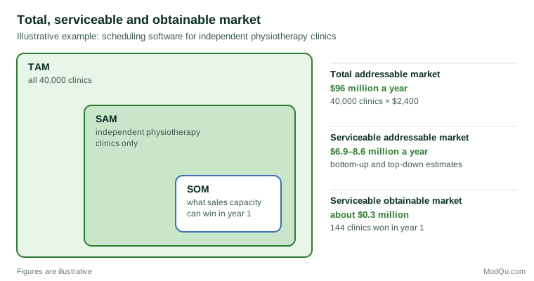
Business plans and investor presentations commonly divide the market into three nested layers (Figure 1):
- Total addressable market (TAM): the total demand for the product category in the defined market, if every possible customer bought.
- Serviceable addressable market (SAM): the part of the TAM that the business can actually serve, given its product, price, channels and geography.
- Serviceable obtainable market (SOM): the part of the SAM the business can realistically win within a stated period, given competition and its own resources.
The SOM is the figure that matters for planning revenue. A common weakness in business plans is to present a very large TAM and then assume that the business will capture a small percentage of it. "If we get just 1% of a $10 billion market" is not an estimate; it gives no reason to believe that 1% is achievable. A credible SOM is built from evidence about how many customers the business can reach, convert and keep.
Top-down sizing
Top-down sizing starts with a large, known total and narrows it through a series of percentages to the market of interest. The total might be population, the number of households, the number of businesses in an industry, or total spending in a broad category from official statistics or industry reports. Each step applies a ratio: the share of households with a relevant characteristic, the share that use the type of product, the share in the target price range, and so on. This structure is sometimes called the chain-ratio method (Kotler & Keller, 2016).
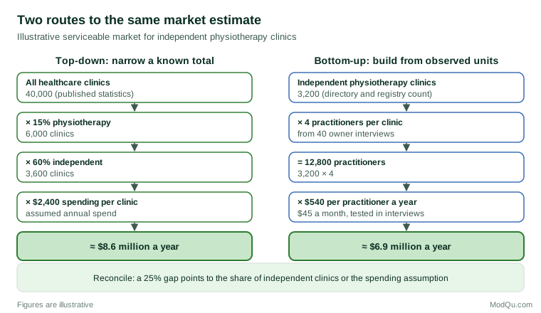
Consider an illustrative example: a company plans to sell scheduling software to independent physiotherapy clinics in a country with 40,000 healthcare clinics of all kinds.
- Total clinics: 40,000.
- Share that are physiotherapy clinics: 15%, giving 6,000.
- Share that are independent rather than part of a chain using central software: 60%, giving 3,600.
- Expected annual spending per clinic on scheduling software: $2,400.
- Serviceable market: 3,600 × $2,400 = about $8.6 million a year.
If every one of the 40,000 clinics bought scheduling software at the same spending, the total addressable market would be 40,000 × $2,400 = $96 million a year. That figure describes the whole category; the $8.6 million is the part this company, which serves only independent physiotherapy clinics, can address.
Top-down sizing is quick and uses published data. Its weaknesses are that each ratio carries uncertainty, that errors multiply across the chain, and that the ratios are often borrowed from other markets or guessed. A chain of five ratios, each of which could be 20% too high, can produce a result that is about two and a half times too high. Top-down estimates also say little about how customers buy, which is what a business needs to know to plan its sales.
Bottom-up sizing
Bottom-up sizing builds the estimate from units the researcher can observe: individual customers, transactions or sales outlets. It multiplies the number of buying units by the quantity each buys and the price per unit. The inputs come from primary research, such as customer interviews and surveys, and from the company's own data, such as early sales, pilot results or pricing tests.
For the same physiotherapy example, a bottom-up estimate might proceed as follows:
- A count of independent physiotherapy clinics from a professional association directory and business registry: 3,200.
- Interviews with 40 clinic owners show an average of 4 practitioners per clinic.
- Price tested in the interviews: $45 per practitioner per month, or $540 per practitioner a year.
- Serviceable market: 3,200 × 4 × $540 = about $6.9 million a year.
The two estimates differ by about 25%. The difference is informative. It shows that the top-down ratio for independent clinics, or the assumed spending per clinic, may be too high. Reconciling the two, by finding which inputs explain the gap, usually improves both.
A bottom-up estimate can then be carried through to an obtainable market by adding the business's own sales capacity and conversion rates. If the company's two salespeople can each hold 30 demonstrations a month, and pilot work suggests that one demonstration in five leads to a sale, the company can win about 144 clinics a year, or roughly $310,000 in annual revenue at the tested price after one year. This figure rests on the company's real constraints rather than on an assumed market share, and it shows directly what would need to change, such as more salespeople or a higher conversion rate, to grow faster.
Choosing between the approaches
The two approaches suit different situations:
- Top-down suits early screening of many opportunities, markets with good published statistics, and situations where a rough order of magnitude is enough to make a decision.
- Bottom-up suits business plans, sales planning and investment decisions, markets with poor published data, and new products for which no category totals exist.
Armstrong (2001), summarising forecasting research, recommends using several methods that draw on different information and combining their results. Combining reduces error because the methods do not share all their weaknesses. In market sizing, the practical version of this advice is to produce both a top-down and a bottom-up estimate, compare them, and investigate any large difference before relying on either.
Sources of input data
Top-down estimates draw mostly on secondary sources: national statistics agencies, census data, business registers, trade association figures, company annual reports and published industry reports. Each source should be checked for its definition of the market, its date and its method. Commercial industry reports often give a single headline figure without explaining how it was produced. Two reports on the "same" market can differ several-fold because they define it differently.
Bottom-up estimates draw mostly on primary research: counts of potential customers from directories and registers, interviews and surveys to establish usage and spending, and price testing. Where the company already sells, its own transaction data are the most reliable input.
When data are scarce, estimates can be built from reasoned assumptions, a technique often called Fermi estimation after the physicist Enrico Fermi, who was known for making quick, reasonable estimates from very little information. Weinstein and Adam (2008) show how breaking a question into parts that can each be estimated separately produces answers that are often within a reasonable range, because errors in individual parts tend partly to cancel. The method is useful for a first check but should be replaced by data wherever data can be obtained.
Using surveys of purchase intention
Surveys are often used to estimate how many customers would buy a product. They need careful interpretation. People who say they will buy usually buy at lower rates than they predict, and the gap differs between products and situations.
Juster (1966) found that asking respondents to state the probability that they would buy, on an eleven-point scale from "certainly not" to "certainly," predicted actual purchases better than asking whether they intended to buy. Jamieson and Bass (1989) compared methods for adjusting stated intentions and showed that the raw figures need correction before they are used to estimate trial. Morwitz et al. (2007) found that intentions predict sales more accurately for existing products than for new ones, for durable goods than for non-durables, and over short periods than over long ones. Armstrong et al. (2000) found that, for existing products, adding intentions data to a forecast improved its accuracy.
In practice, analysts apply a conversion factor to stated intentions, such as counting only a proportion of those who say they "definitely would buy." The factor should come from evidence: the company's past launches, published category norms or a pilot sale. A survey result used without such adjustment will usually overstate demand.
Sizing markets that do not yet exist
Products that create a new category present a particular difficulty: there is no current market to measure. The question becomes how many customers could eventually adopt the product, and how quickly. Three approaches are common.
Analogies. The researcher identifies an earlier product that faced a similar adoption situation, such as similar price, similar benefit and similar need to change behaviour, and uses its adoption history as a guide. Lilien et al. (1992) and Urban and Hauser (1993) describe how analogies are chosen and applied in marketing models.
Diffusion models. The Bass (1969) model describes adoption as driven by external influence, such as advertising, and by internal influence from earlier adopters. Its parameters cannot be estimated from a product's own sales before launch, so they are taken from analogous products or from published averages. Sultan et al. (1990) combined 213 applications of the model and reported average values that are often used as starting points. Van den Bulte and Stremersch (2004) found that the relative strength of the two influences varies between countries. Mahajan et al. (1990) review the model's extensions. The third input, the eventual number of adopters, comes from market sizing itself.
Time to takeoff. New categories often sell slowly for years before sales rise sharply. Golder and Tellis (1997) studied really new consumer durables in the United States and found that, for categories introduced after the Second World War, the time from introduction to the point at which sales take off averaged about six years, and that takeoff was associated with falling prices. Rogers (2003) describes how adoption spreads through groups of innovators, early adopters, an early and late majority and laggards. Moore (1991) argued that for technology products there is a gap between early adopters and the mainstream market that many products fail to cross. All three point to the same practical lesson: the size of a new market and the speed at which it is reached are separate questions, and a large eventual market does not mean early revenue.
Bias in market estimates
Market estimates are prone to optimism. Kahneman and Lovallo (1993) described how planners take an "inside view," building a forecast from the details of their own project, and neglect the "outside view," which asks how similar projects have turned out. The inside view tends to produce bold forecasts. Lovallo and Kahneman (2003) recommended reference class forecasting: identifying a group of comparable past projects and starting from their actual results before adjusting for the specific case. Buehler et al. (1994) showed the same pattern in a different setting: people consistently underestimated how long their own tasks would take, even when they knew that similar tasks had taken longer in the past.
Anchoring is a second source of bias. Tversky and Kahneman (1974) showed that numerical estimates are pulled toward a starting value, even an irrelevant one. In market sizing, a headline figure from an industry report can anchor every later step. Building the bottom-up estimate independently, before looking at the top-down result, reduces this effect.
Tetlock and Gardner (2015) found that the most accurate forecasters in long-running forecasting tournaments routinely began with base rates from comparable cases and then adjusted for specifics, broke questions into parts, and updated their estimates as new information arrived. The same habits suit market sizing.
Checking an estimate
A market estimate is ready to use only after it has been checked. The following tests catch most errors:
- Triangulate. Compare top-down and bottom-up estimates and explain any large gap.
- Test against reality. Compare the implied number of customers with known figures, such as the number of businesses in the industry, or the implied spending with what customers report they spend.
- Check the arithmetic and units. Annual and monthly figures, revenue and units, and different currencies are frequently mixed.
- Run a sensitivity analysis. Change each key input to its plausible low and high values and see how much the result moves. Inputs that move the result most deserve the most research.
- Present a range. Report low, central and high estimates with the assumptions behind each, instead of a single precise figure that implies more certainty than exists.
- Document sources. Record where each input came from and its date, so that the estimate can be checked and updated.
Summary
Market sizing starts with a precise definition of the product, customers, geography, period and unit. Top-down methods narrow a known total through a chain of ratios; bottom-up methods build from counts of customers, their usage and price. Each has weaknesses, and using both, then reconciling the difference, gives a more reliable estimate than either alone. Survey intentions need adjustment before they are used to estimate demand, and new categories require analogies and diffusion models, with separate attention to how quickly the market will develop. Because estimates are prone to optimism and anchoring, they should start from comparable cases, be tested for sensitivity, and be presented as ranges with their assumptions stated.
References
Armstrong, J. S. (Ed.). (2001). Principles of forecasting: A handbook for researchers and practitioners. Kluwer Academic.
Armstrong, J. S., Morwitz, V. G., & Kumar, V. (2000). Sales forecasts for existing consumer products and services: Do purchase intentions contribute to accuracy? International Journal of Forecasting, 16(3), 383–397.
Bass, F. M. (1969). A new product growth for model consumer durables. Management Science, 15(5), 215–227. https://doi.org/10.1287/mnsc.15.5.215
Buehler, R., Griffin, D., & Ross, M. (1994). Exploring the "planning fallacy": Why people underestimate their task completion times. Journal of Personality and Social Psychology, 67(3), 366–381.
Day, G. S., Shocker, A. D., & Srivastava, R. K. (1979). Customer-oriented approaches to identifying product-markets. Journal of Marketing, 43(4), 8–19.
Golder, P. N., & Tellis, G. J. (1997). Will it ever fly? Modeling the takeoff of really new consumer durables. Marketing Science, 16(3), 256–270.
Jamieson, L. F., & Bass, F. M. (1989). Adjusting stated intention measures to predict trial purchase of new products: A comparison of models and methods. Journal of Marketing Research, 26(3), 336–345. https://doi.org/10.2307/3172905
Juster, F. T. (1966). Consumer buying intentions and purchase probability: An experiment in survey design. Journal of the American Statistical Association, 61(315), 658–696.
Kahneman, D., & Lovallo, D. (1993). Timid choices and bold forecasts: A cognitive perspective on risk taking. Management Science, 39(1), 17–31.
Kotler, P., & Keller, K. L. (2016). Marketing management (15th ed.). Pearson.
Lilien, G. L., Kotler, P., & Moorthy, K. S. (1992). Marketing models. Prentice Hall.
Lovallo, D., & Kahneman, D. (2003). Delusions of success: How optimism undermines executives' decisions. Harvard Business Review, 81(7), 56–63.
Mahajan, V., Muller, E., & Bass, F. M. (1990). New product diffusion models in marketing: A review and directions for research. Journal of Marketing, 54(1), 1–26. https://doi.org/10.1177/002224299005400101
Moore, G. A. (1991). Crossing the chasm: Marketing and selling technology products to mainstream customers. HarperBusiness.
Morwitz, V. G., Steckel, J. H., & Gupta, A. (2007). When do purchase intentions predict sales? International Journal of Forecasting, 23(3), 347–364.
Rogers, E. M. (2003). Diffusion of innovations (5th ed.). Free Press.
Sultan, F., Farley, J. U., & Lehmann, D. R. (1990). A meta-analysis of applications of diffusion models. Journal of Marketing Research, 27(1), 70–77.
Tetlock, P. E., & Gardner, D. (2015). Superforecasting: The art and science of prediction. Crown.
Tversky, A., & Kahneman, D. (1974). Judgment under uncertainty: Heuristics and biases. Science, 185(4157), 1124–1131.
Urban, G. L., & Hauser, J. R. (1993). Design and marketing of new products (2nd ed.). Prentice Hall.
Van den Bulte, C., & Stremersch, S. (2004). Social contagion and income heterogeneity in new product diffusion: A meta-analytic test. Marketing Science, 23(4), 530–544.
Weinstein, L., & Adam, J. A. (2008). Guesstimation: Solving the world's problems on the back of a cocktail napkin. Princeton University Press.