
Insights · Insight quality and pitfalls
Overgeneralisation From Small or Unrepresentative Samples
Why conclusions drawn from small or unrepresentative samples so often fail to hold, covering the "law of small numbers", the extreme results small groups produce, selection and nonresponse bias, the big data paradox, and practical checks before generalising a finding.
An insight is useful only if it holds beyond the people or cases it was drawn from. A finding from twelve interviews, one store, a survey of website visitors or a pilot in a single region is often reported as though it described all customers, all stores or the whole market. Sometimes it does. Often it does not. Overgeneralisation, drawing broad conclusions from samples that are too small or not representative, is one of the most common ways in which apparently solid insights turn out to be wrong. This article explains why it happens and how to guard against it.
The law of small numbers
Tversky and Kahneman (1971) found that even trained researchers expected small samples to resemble the population they came from much more closely than statistics would predict. They called this belief the "law of small numbers", a play on the law of large numbers, which holds only for large samples. Researchers in their study were too confident in results from small samples, underestimated how much those results would vary in a replication, and attributed unexpected differences to real causes rather than to chance. Kahneman and Tversky (1972) showed that people judge the likelihood of a sample by how well it represents the population, largely ignoring sample size.
The practical consequence is that small samples feel more informative than they are. A finding that eight of ten customers prefer a new design seems decisive, but with ten people the true share could plausibly be anywhere from about 50% to 95%.
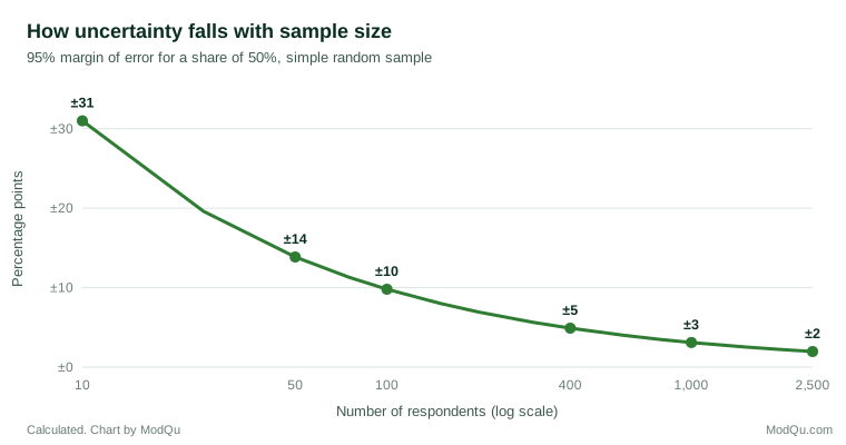
Small groups produce extreme results
Small samples are not only less precise; they produce extreme results more often. Wainer (2007) described the formula for the standard error of a mean, which shows that variation in averages shrinks with the square root of sample size, as "the most dangerous equation" because ignoring it has led to costly mistakes. Wainer's best-known example concerns schools. Analyses showed that small schools were over-represented among the highest-performing schools, which encouraged large investments in creating smaller schools. But small schools were also over-represented among the worst performers, because small groups vary more. Wainer and Zwerling (2006) showed that once size was taken into account, there was no evidence that smaller schools produced better results.
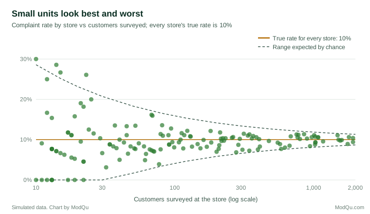
The same pattern appears in business data. Rankings of stores, sales territories, products or campaigns by a rate, such as conversion, complaints or growth, will tend to put small units at both the top and the bottom. An analyst who studies the top-performing stores to find the secret of their success may simply be studying the smallest stores.
Small studies and exaggerated effects
Small samples also distort the size of effects. Button et al. (2013) showed that many neuroscience studies had low statistical power, and explained that when such studies do find an effect, its size is likely to be exaggerated. Gelman and Carlin (2014) described this as a "Type M" or magnitude error: when a small study produces a statistically significant result, the estimated effect is often much larger than the true one, and can even have the wrong sign. Ioannidis (2005) argued that small studies, small effects and flexible analysis all increase the chance that a published finding is false.
For insight work, this means that striking results from small pilots, tests or samples should be expected to shrink when tested at scale. Cumming (2014) recommended reporting estimates with confidence intervals rather than relying on whether a result is significant, so that readers can see how uncertain an estimate is.
Unrepresentative samples
Size is not the only problem. A large sample can be badly unrepresentative. The most famous example is the 1936 United States presidential election poll by the Literary Digest magazine, which collected over two million responses and predicted a clear win for the losing candidate. Squire (1988) analysed survey data from the time and concluded that the poll failed mainly because of who responded: supporters of the losing candidate were more likely to return their ballots, and the initial sample was also skewed.
Unrepresentative samples are common in insight work. Customers who answer surveys differ from those who do not. Website visitors differ from the wider market. Online panels differ from the general population. Henrich et al. (2010) pointed out that most psychology research had been conducted with people from Western, educated, industrialised, rich and democratic societies, and that findings from these samples often did not hold elsewhere. Sears (1986) raised similar concerns about the heavy reliance of social psychology on university students.
Nonresponse can bias results even when the initial sample is good. Groves (2006) showed that the bias depends on whether the reasons for not responding are related to the variable being measured, not on the response rate alone. Groves and Peytcheva (2008) conducted a meta-analysis and found that response rates were only weakly related to the size of nonresponse bias, so a high response rate does not guarantee representative results and a low one does not guarantee bias.
Subgroups within large samples
A sample that is large overall can still be small where it matters. A survey of 1,000 customers may include only 60 in a particular region or 40 who bought a premium product. Comparisons between such subgroups are much less precise than the headline figures, and differences of ten points or more can arise by chance. Reports often present subgroup results in the same tables as overall results, with no indication that some are based on very few people.
The risk grows when many subgroups are compared. With twenty regions, a few will show unusual results by chance alone, and these are exactly the results that attract attention. Good practice is to show the number of respondents behind each subgroup figure, to suppress or flag figures based on very small numbers, and to treat differences found by scanning many subgroups as hypotheses to be confirmed rather than as findings.
Qualitative samples
Qualitative research uses small samples deliberately, and rightly so: its aim is to understand experiences, meanings and mechanisms in depth, not to estimate how common they are. Guest et al. (2006) found in one study that most themes appeared within the first twelve interviews, which supports the use of modest samples for discovering what matters to people. The problem arises when qualitative findings are reported as though they were estimates: "most customers feel..." based on eight interviews, or a theme presented as dominant because it came up often in a small, purposive sample.
Qualitative findings generalise in a different way. They can show that something exists, how it works and what it means to the people involved, and they can suggest that it may occur in similar settings. Claims about how widespread it is need a different kind of evidence, usually a survey designed to represent the population.
The big data paradox
Large data sets can create a false sense of security. Meng (2018) showed mathematically that the error of an estimate from a non-random sample depends on the correlation between whether someone is included and the value being measured, and that even a tiny correlation can produce large errors when the population is large. A non-random sample of millions can be less accurate than a random sample of a few hundred. Bradley et al. (2021) demonstrated this "big data paradox" with surveys of COVID-19 vaccine uptake in the United States: two very large online surveys, with hundreds of thousands of respondents, substantially overestimated vaccine uptake compared with official figures, while a much smaller survey designed to be representative was more accurate.
Non-probability samples are not useless. Wang et al. (2015) showed that a large, unrepresentative poll of video game users could produce accurate election forecasts after statistical adjustment to match the population. Yeager et al. (2011) compared probability and non-probability surveys and found that the probability samples were generally more accurate, even after weighting, though non-probability samples varied in quality. Baker et al. (2013) reviewed non-probability sampling for a professional association and concluded that such samples can be useful for some purposes, but that their accuracy depends on assumptions that should be stated and tested.
Checks before generalising
Several questions help decide whether a finding can be generalised.
How large is the sample, and how uncertain is the estimate? Report confidence intervals or ranges, not only point estimates.
Who is in the sample, and who is not? Compare the sample with the population on known characteristics, such as age, region and customer value, and consider whether those missing might differ on the measure of interest.
Why did people take part? Self-selected samples, such as people who chose to answer a survey or post a review, are likely to differ from those who did not.
Are small units being ranked? When comparing rates across stores, products or regions, plot them against size and expect the smallest to appear at both extremes.
Has the finding been replicated? A result seen in one sample should be confirmed in another before large decisions depend on it.
Is the claim proportionate to the evidence? Qualitative research with a small purposive sample can show what exists and why; it cannot show how common it is. Kish (1965) set out the principles of sampling that allow estimates to be generalised to a population, and claims about prevalence require samples designed with those principles in mind.
An example
Consider a hypothetical restaurant chain that pilots a new menu in three restaurants. Sales per customer rise by 15% in the pilot, and the board approves a national rollout. After rollout, sales per customer rise by only 3%.
Looking back, the problems are clear. Three restaurants is a very small sample, and the three were chosen because their managers were enthusiastic, which may have affected how the menu was presented. The pilot ran during a period when those restaurants were busier than usual. And the effect estimated from such a small pilot was likely to be exaggerated even if the restaurants had been typical. A larger pilot, with restaurants chosen at random and compared with similar restaurants that kept the old menu, would have given a more realistic estimate. So would a simple check before rollout: plotting the change in sales per customer for every restaurant in the chain over the same period would have shown that several restaurants without the new menu had also seen double-digit rises, a sign that the pilot result was within the range of ordinary variation.
The chain now runs pilots in at least twenty restaurants, chosen at random from a list of those able to take part, with a matched set of comparison restaurants. Pilot results are reported as a range rather than a single figure, and the board is told in advance that the national effect is likely to be smaller than the pilot estimate. These changes have made pilots less exciting but much more reliable as a guide to decisions.
Key takeaways
People expect small samples to resemble the population more closely than they do, and small groups produce extreme results more often than large ones. Effects estimated from small studies are often exaggerated. Large samples can also mislead if they are not representative, and in large populations even a small selection bias can produce large errors. Before generalising, check the size and uncertainty of the estimate, who is and is not in the sample, why people took part, whether small units are being ranked, and whether the finding has been replicated.
References
Baker, R., Brick, J. M., Bates, N. A., Battaglia, M., Couper, M. P., Dever, J. A., Gile, K. J., & Tourangeau, R. (2013). Summary report of the AAPOR task force on non-probability sampling. Journal of Survey Statistics and Methodology, 1(2), 90–143. https://doi.org/10.1093/jssam/smt008
Bradley, V. C., Kuriwaki, S., Isakov, M., Sejdinovic, D., Meng, X.-L., & Flaxman, S. (2021). Unrepresentative big surveys significantly overestimated US vaccine uptake. Nature, 600(7890), 695–700. https://doi.org/10.1038/s41586-021-04198-4
Button, K. S., Ioannidis, J. P. A., Mokrysz, C., Nosek, B. A., Flint, J., Robinson, E. S. J., & Munafò, M. R. (2013). Power failure: Why small sample size undermines the reliability of neuroscience. Nature Reviews Neuroscience, 14(5), 365–376. https://doi.org/10.1038/nrn3475
Cumming, G. (2014). The new statistics: Why and how. Psychological Science, 25(1), 7–29. https://doi.org/10.1177/0956797613504966
Gelman, A., & Carlin, J. (2014). Beyond power calculations: Assessing Type S (sign) and Type M (magnitude) errors. Perspectives on Psychological Science, 9(6), 641–651. https://doi.org/10.1177/1745691614551642
Groves, R. M. (2006). Nonresponse rates and nonresponse bias in household surveys. Public Opinion Quarterly, 70(5), 646–675. https://doi.org/10.1093/poq/nfl033
Groves, R. M., & Peytcheva, E. (2008). The impact of nonresponse rates on nonresponse bias: A meta-analysis. Public Opinion Quarterly, 72(2), 167–189. https://doi.org/10.1093/poq/nfn011
Guest, G., Bunce, A., & Johnson, L. (2006). How many interviews are enough? An experiment with data saturation and variability. Field Methods, 18(1), 59–82. https://doi.org/10.1177/1525822X05279903
Henrich, J., Heine, S. J., & Norenzayan, A. (2010). The weirdest people in the world? Behavioral and Brain Sciences, 33(2–3), 61–83. https://doi.org/10.1017/S0140525X0999152X
Ioannidis, J. P. A. (2005). Why most published research findings are false. PLoS Medicine, 2(8), Article e124. https://doi.org/10.1371/journal.pmed.0020124
Kahneman, D., & Tversky, A. (1972). Subjective probability: A judgment of representativeness. Cognitive Psychology, 3(3), 430–454. https://doi.org/10.1016/0010-0285(72)90016-3
Kish, L. (1965). Survey sampling. Wiley.
Meng, X.-L. (2018). Statistical paradises and paradoxes in big data (I): Law of large populations, big data paradox, and the 2016 US presidential election. Annals of Applied Statistics, 12(2), 685–726. https://doi.org/10.1214/18-AOAS1161SF
Sears, D. O. (1986). College sophomores in the laboratory: Influences of a narrow data base on social psychology's view of human nature. Journal of Personality and Social Psychology, 51(3), 515–530. https://doi.org/10.1037/0022-3514.51.3.515
Squire, P. (1988). Why the 1936 Literary Digest poll failed. Public Opinion Quarterly, 52(1), 125–133. https://doi.org/10.1086/269085
Tversky, A., & Kahneman, D. (1971). Belief in the law of small numbers. Psychological Bulletin, 76(2), 105–110. https://doi.org/10.1037/h0031322
Wainer, H. (2007). The most dangerous equation. American Scientist, 95(3), 249–256. https://doi.org/10.1511/2007.65.249
Wainer, H., & Zwerling, H. L. (2006). Evidence that smaller schools do not improve student achievement. Phi Delta Kappan, 88(4), 300–303. https://doi.org/10.1177/003172170608800411
Wang, W., Rothschild, D., Goel, S., & Gelman, A. (2015). Forecasting elections with non-representative polls. International Journal of Forecasting, 31(3), 980–991. https://doi.org/10.1016/j.ijforecast.2014.06.001
Yeager, D. S., Krosnick, J. A., Chang, L., Javitz, H. S., Levendusky, M. S., Simpser, A., & Wang, R. (2011). Comparing the accuracy of RDD telephone surveys and internet surveys conducted with probability and non-probability samples. Public Opinion Quarterly, 75(4), 709–747. https://doi.org/10.1093/poq/nfr020